
Nominal vs. Nominal
Part 3b: Post-hoc test
On the previous page we saw how to test if there is an association between two nominal variables (or if one might be influencing the other), but what might this association be.
There are a few different ways to perform a so-called post-hoc analysis. A nice article explaining some of them can be found in an article by Sharpe (2015). I will focus on two methods.
First we might simply look at the differences between the observed and the expected counts for each cell. However imagine a cell that has an observed count of 80 and an expected count of 70, that is a difference of 10 but does not seem like a lot, while another cell has an observed count of 5 and an expected count of 15, then the 10 difference does seem like a lot. To account for these many authors will suggest to look at either so called adjusted residuals, or Pearson residuals, or adjusted standardized residuals. These standardized residuals can then be used to test if the observed and expected value in the population might actually be different as well.
In below the adjusted residuals in the example.
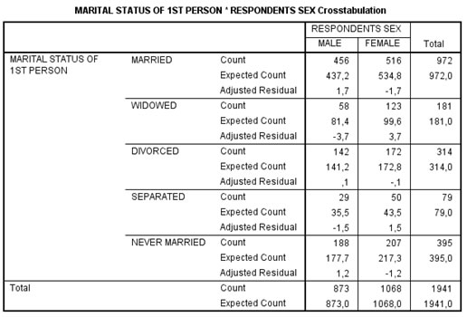
The adjusted residuals seem to be highest for widowed. At 95% confidence level if the value is above 1.96 or below -1.96 it could be considered significantly different, but since we are doing this for each cell we actually have a big risk in making the wrong decision. To adjust for this multiple testing we should adjust the significance level by dividing the original 0.05 level by the number of tests we perform (in this case the number of cells). In the example we should therefor look at a significance of 0.05 / 10 = 0.05, which would correspond to a critical value of 2.81 (or below -2.81). This is known as a Bonferroni correction. To help with determining this critical value I've created a small Excel tool, which can be downloaded here.
In the example the Widowed adjusted residual is the only one that is above this adjusted significance level. We could add this to our report.
Gender and marital status showed to have a significant association, χ2(4, N = 1941) = 16.99, p < .001. A post-hoc z-test on the adjusted residuals with Bonferroni correction revealed that only for widowed there was a significant difference between the male and female percentage, p < .05.
Click here on how to determine the adjusted residuals, with SPSS, R (Studio), Excel, or Python.
with SPSS
with R (Studio)
with Excel
with Python
An alternative method to perform the post-hoc test is to collapse the cross table into every possible 2x2 table. In this example there are only two columns, so this leaves the 5 rows. With collapsing is meant to for example then look at the results of the Pearson chi-square test results of married vs. the rest, then widowed vs. the rest, etc. This is sometimes known as a column proportion test. Click below to see how to perform this kind of post-hoc analysis
The results of this post-hoc test can be reported in a similar way as the previous method.
Gender and marital status showed to have a significant association, χ2(4, N = 1941) = 16.99, p < .001. A pairwise z-test post hoc analysis with Bonferroni correction revealed that only for widowed there was a significant difference between the male and female percentage, p < .05.
Click here to see how to obtain the column proportion test with SPSS
Two different methods to perform this test with SPSS
via Crosstabs
via Custom tables
As a last step in the analyses we can have a look at how strong the association is between the two variables, which will be discussed on the next page.
Two nominal variables
![]()

Google adds