
Analysing a single ordinal variable
2a: Test for median (one-sample Wilcoxon signed rank test)
From the results in the previous parts we noticed in the example that not many people think accounting is scientific. However that was just based on a sample, and we would like to know how this would be in the population. Would the majority of people in the population also not see accounting as very scientific? The majority would be more than 50% of the people, so in other words, is the median (the score in the middle) in the populaiton significantly different from 2.5 (since 2 = pretty scientific, and 3 = not scientific)?
Two tests could be used for this, the first does exactly what is described above, and is known as a sign-test, however another test is more frequently used and has a lot scarier name: one-sample Wilcoxon signed rank test (Wilcoxon, 1945). This second test uses rankings (it ranks the scores) and because of this might give a slightly different result. The advantage of this second test is that it can catch some smaller differences and is the one I will explain here. If you are curious about what the Wilcoxon test does exactly I'd recommend this site. The appendix at the bottom of the page has some more information about the sign-test in case you are curious about it.
The significance of the Wilcoxon signed rank test will tell us how likely it is to have a result as in our sample, or even more extreme if the median in the population is indeed a certain value (in the example we use 2.5). If this chance is very low, the population mos likely has another median than the one expected.
In the example the significance is .000, which is usually considered very low. This indicates that the median is significantly different from 2.5, so it is unlikely that the median in the population is 2.5. In the report the results of the test could for example go like:
A one-sample Wilcoxon signed-rank test indicated that the median was significantly different from 2.5, Z = 11.93, p < .001.
Click here to see how you can perform a one-sample Wilcoxon signed rank test.
with Excel
Excel file from video: TS - One-Sample Wilcoxon.xlsm.
with Flowgorithm
exact test
WARNING: This very quickly becomes too large in computation that Flowgorithm can handle.
A flowgorithm for the exact one-sample Wilcoxon signed rank test is shown in Figure 1.
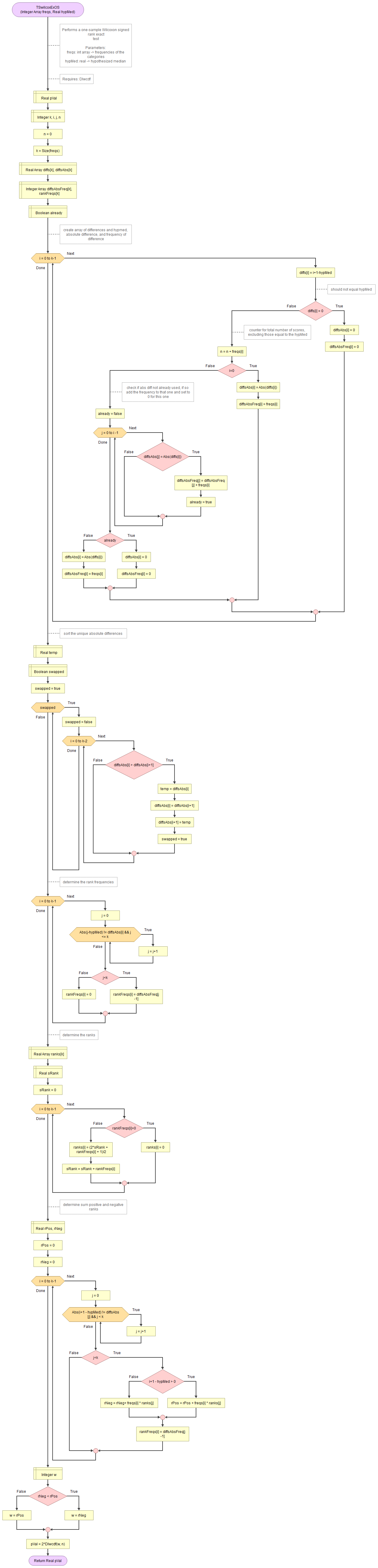
It takes as input an array of integers with the observed frequencies and the hypothesized median.
It uses the function for Wilcoxon distribution which in turn uses the permutation distribution and the binomial coefficient.
Flowgorithm file: FL-TSwilcoxOSexact.fprg.
normal approximation
A flowgorithm for the one-sample Wilcoxon signed rank test using the normal approximation is shown in Figure 2.
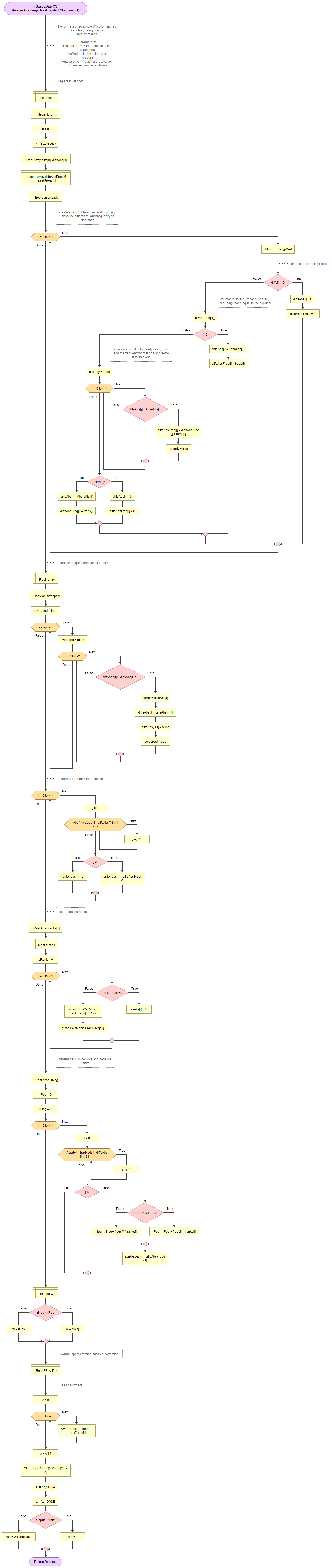
It takes as input an array of integers with the observed frequencies, the hypothesized median, and a string to indicate if you want to see the z-value or the p-value.
It uses the function for standard normal cumulative distribution.
Flowgorithm file: FL-TSwilcoxOSappr.fprg.
with Python
Jupyter Notebook used in video: TS - Wilcoxon One-Sample.ipynb.
Data file used in video and notebook GSS2012a.csv.
with R (Studio)
click on the thumbnail below to see where to find the values used in the report.
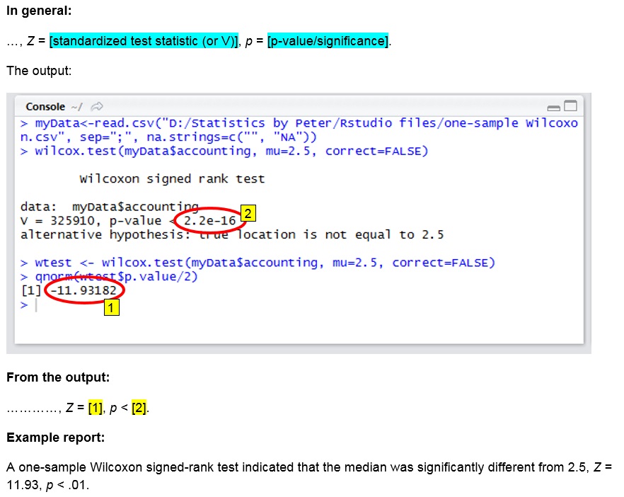
R script used in video: TS - One-Sample Wilcoxon.R.
Data file used in video and notebook GSS2012a.csv.
with SPSS
watch the video below, or download the pdf instructions (via bitly, opens in new window/tab).
click on the thumbnail below to see where to find the values used in the report.
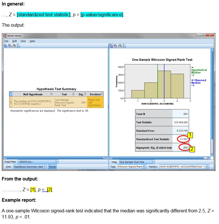
Datafile used in video: GSS2012-Adjusted.sav
Manually (formulas and example)
Formulas
The unadjusted test statistic is given by:
\( W=\sum_{i=1}^{n_{r}^{+}}r_{i}^{+} \)
In this formula \( n_{r}^{+}\) is the number of ranks with a positive deviation from the hypothesized median, and \(r_{i}^{+}\) the i-th rank of of the ranks with a positive deviation from the hypothesized median.
The ranks are based on the absolute deviation of each score with the hypothesized median, removing scores that are equal to the hypothesized median. In formula notation we could determine the sequence of ranks as:
\(r=\textup{rank}(|d|)\)
Where d is the sequence of:
\(d_{i}=y_{i}-\theta\)
Where θ is the hypothesized median, and and y the sequence of original scores, but with the scores removed that equal θ
To adjust for ties we need a few more things.
The variance is given by:
\( s^{2}=\frac{n_{r}\times\left(n_{r}+1\right)\times\left(2\times n_{r}+1\right)}{24} \)
Where nr is the number of ranks.
The adjustment is given by:
\(A=\frac{\sum_{i=1}^{n_f}\left(t_i^3-t_i\right)}{48}\)
In this formula ti is the number of ties for each unique ranks i, and nf the number of unique ranks.
The adjusted variance then becomes:
\(s_*^2=s^2-A\)
The adjusted standard error:
\(SE_*=\sqrt{s_*^2}\)
Another small adjustment is needed:
\(D=\frac{n_r\times\left(n_r+1\right)}{4}\)
Finally the adjusted W statistics is then:
\(W_*=\frac{W-D}{SE_*}\)
Example
We are given six scores from an ordinal scale and like to test if the median is significantly different from 3. The six scores are:
\(x=\left(4,4,5,1,5,3 \right)\)
The hypothesized median was given to be 3, so:
\(\theta=3\)
First we now remove any score from x that is equal to the hypothesized median, which in the example is only the last score. So we set:
\(y=\left(4,4,5,1,5\right)\)
Then we determine the difference with the hypothesized median:
\(d=\left(4-3,4-3,5-3,1-3,5-3\right)=\left(1,1,2,-2,2\right)\)
To determine the ranks, we need tha absolute values of these:
\(|d|=\left(|1|,|1|,|2|,|-2|,|2|\right)=\left(1,1,2,2,2\right)\)
Then we rank these absolute differences. The lowest score is a 1, but this occurs twice. So they take up rank 1 and 2, or on average rank 1.5. Then we have a score of 2, but this occurs three times. So they take ranks 3, 4 and 5, or on average rank 4. It is these average ranks that we need:
\(r=\left(1.5,1.5,4,4,4\right)\)
To determine the unadjusted W we sum up the ranks, but only for those that had a positive deviation (from d). The fourth entry in d is negative (-2), so we do not add the rank of 4 from that score. We therefor get:
\(W=1.5+1.5+4+4=11\)
We have five ranks so nr = 5, so we can also determine the variance:
\(s^2=\frac{n_{r}\times\left(n_{r}+1\right)\times\left(2\times n_{r}+1\right)}{24} =\frac{5\times\left(5+1\right)\times\left(2\times 5+1\right)}{24}\)
\(=\frac{5\times6\times\left(10+1\right)}{24}=\frac{5\times6\times11}{24}=\frac{330}{24}=\frac{55}{4}=13.75\)
We have a rank of 1.5 that occurs twice, and a rank of 4 that occurs three times. Therefore:
\(A=\frac{\sum_{i=1}^{n_f}\left(t_i^3-t_i\right)}{48}=\frac{\left(2^3-2\right)+\left(3^3-3\right)}{48} =\frac{\left(8-2\right)+\left(27-3\right)}{48} =\frac{6+24}{48}\)
\(=\frac{30}{48}=\frac{5}{8}=0.625\)
The adjusted variance then becomes:
\(s_*^2=s^2-A=\frac{55}{4}-\frac{5}{8}=\frac{55\times2}{4\times2}-\frac{5}{8}\)
\(=\frac{110}{8}-\frac{5}{8}=\frac{110-5}{8}=\frac{105}{8}=13.125\)
The adjusted standard error:
\(SE_*=\sqrt{s_*^2}=\sqrt\frac{105}{8}=\frac{1}{8}\sqrt{105\times8}=\frac{1}{8}\sqrt{840}\)
\(=\frac{1}{8}\sqrt{4\times210}=\frac{1}{8}\times\sqrt{4}\times\sqrt{210}=\frac{1}{8}\times2\times\sqrt{210}=\frac{1\times2}{8}\times\sqrt{210}\)
\(=\frac{2}{8}\times\sqrt{210}=\frac{1}{4}\sqrt{210}\approx3.623\)
The other small adjustment:
\(D=\frac{n_r\times\left(n_r+1\right)}{4}=\frac{5\times\left(5+1\right)}{4}=\frac{5\times6}{4}=\frac{30}{4}=\frac{15}{2}=7.5\)
The adjusted W statistic becomes:
\(W_*=\frac{W-D}{SE_*}=\frac{11-\frac{15}{2}}{\frac{1}{4}\sqrt{210}} =\frac{\frac{22}{2}-\frac{15}{2}}{\frac{\sqrt{210}}{4}} =\frac{\frac{22-15}{2}}{\frac{\sqrt{210}}{4}} =\frac{\frac{7}{2}}{\frac{\sqrt{210}}{4}}\)
\(=\frac{7\times4}{\sqrt{210}\times2} =\frac{7\times2}{\sqrt{210}} =\frac{14}{\sqrt{210}} =\frac{14}{\sqrt{210}}\times\frac{\sqrt{210}}{\sqrt{210}}\)
\(=\frac{14\times\sqrt{210}}{\sqrt{210}\times\sqrt{210}} =\frac{14\times\sqrt{210}}{210} =\frac{14\times\sqrt{210}}{14\times15} =\frac{\sqrt{210}}{15}\approx0.966\)
To determine the two-tailed significance either the exact Wilcoxon distribution is used, or if there is sufficient data the standard normal distribution is used.
The next step is to determine if the difference is also a 'big' difference, known as an effect size. This will be the topic for the next part.
Appendix: one-sample sign test (click to expand)
As mentioned at the start of this page, an alternative option might be a so-called one-sample sign test. This test looks only at how many scores are below the expected population median, and how many above. It then uses a binomial test to determine the chance of this. It fully ignores how far from the median each score is. So for example for a sign test with a hypothesized median of 5, it would not matter if the scores were: 3, 3, 4, 4, 4, 5, 5, 9, 10, 15, 22
or : 3, 3, 4, 4, 4, 5, 5, 6, 6, 6, 7, 7
In both examples there are five scores below the expected median, and five above.
Click here to see how you can perform a one-sample sign test
with Excel
Excel file from video: TS - One-Sample Sign.xlsm.
with Flowgorithm
A flowgorithm for the one-sample sign test is shown in Figure 1.
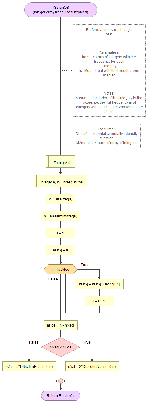
It takes as input an array of integers with the observed frequencies and the hypothesized median.
It uses the function for the binomial cumulative distribution (DIbcdf) and a small helper function to determine the sum of an array. The DIbcdf in turn requires the binomial probability mass function, which in turn uses two helper functions (HEstirlerr and HEbd0). The HEstirlerr function requires the math helper functions factorial and exponential.
Flowgorithm file: FL-TSsignOS.fprg.
with Python
Jupyter Notebook used in video: TS - Sign-test (One-Sample).ipynb.
with R (Studio)
R script used in video: TS - One-Sample Sign Test.R.
Data file used in video and notebook GSS2012-Adjusted.sav.
with SPSS
Datafile used in video: GSS2012-Adjusted.sav
Manually (formula & Example)
The one-sample sign test can be performed using:
\(p = 2\times bcdf\left(n, \text{min}\left(n_+, n_-\right), \frac{1}{2}\right) \)
Where \(bcdf\) is the binomial cumulative distribution function, with \(n\) the number of cases used as number of trials, the minimum of \(n_+\) (the number of cases above the hypothesized median) and \(n_-\) (the number of cases below the hypothesized median) as the number of successes, and 0.5 as the probability of success on each trial.
Example
We are given the results of an ordinal variable as a frequency table shown in Table 1.
| Option | Frequency |
|---|---|
| very scientific | 100 |
| pretty scientific | 199 |
| not too scientific | 348 |
| not scientific at all | 307 |
| Total | 954 |
We would like to know if people tended significantly more towards either end. So, as our hypothesized median we set exactly between 'pretty scientific' and 'not too scientific'
The total number of cases is 954 (\(=n\)). The 'very scientific' and 'pretty scientific' are below the hypothesized median, so \(n_- = 100 + 199 = 299\), and the other two categories are above it, so \(n_- = 348 + 307 = 655\)
Filling out these values in the formula to get the significance we get:
\(p = 2\times bcdf\left(954, \text{min}\left(299, 655\right), \frac{1}{2}\right) = 2\times bcdf\left(954, 299, \frac{1}{2}\right) \approx \frac{2.83}{10^{31}} \)
How to calculate a binomial cumulative density function (bcdf) is explained in the binomial distribution section.
The result in the example is far below the usual threshold of 0.05. The population median is therefor significantly different from the hypothesized one. There is a significant tendency to not see accounting as scientific.
Single ordinal variable
![]()

Google adds