
Analysing a single ordinal variable
2b: Effect size
If a sample size is very large, almost everything will be significant, but perhaps not relevant anymore. It is therefore recommended to also add a so-called effect size measure.
One possible effect size measures that could be suitable for this test, is dividing the z-value by the square root of the sample size (Fritz et al., 2012, p. 12; Mangiafico, 2016; Simone, 2017; Tomczak, M., & Tomczak, E., 2014, p. 23; ).
The formula can be found in Rosenthal book (1991, p. 19) , so I will refer to as the Rosenthal correlation coefficient (as to differentiate it with other correlation coefficients). Probably the original was Cohen (1988, p. 275) who calls it 'f', but all other authors label it 'r'
In the example the standardized test statistic was 11.932 and the sample size was 954 (see output from software used in the previous part). We can then quickly calculate the Rosenthal correlation coefficient: r = 11.932 / SQRT(954) = 0.39. As for the interpretation various rules of thumb exist. One such rule of thumb is from Bartz (1999, p. 184) shown in Table 1.
| Rosenthal Correlation | Interpretation |
|---|---|
0.00 < 0.20 |
very low |
0.20 < 0.40 |
low |
0.40 < 0.60 |
moderate |
0.60 < 0.80 |
strong |
0.80 < 1.00 |
very strong |
| Note: Adapted from Basic statistical concepts (4th ed., p. 19) by A.E. Bartz, 1999, Merill. | |
The 0.39 from the example would then indicate a moderate effect size.
In the report the results of the test we could add this for example like:
A one-sample Wilcoxon signed-rank test indicated that the median was significantly different from 2.5, Z = 11.93, p < .001, with a moderate effect size (r = .39).
Click here to see how you can obtain the Rosenthal Coefficient...
with Excel
Excel file: ES - Rosenthal Correlation.xlsm
with Flowgorithm
A flowgorithm for the Rosenthal Correlation in Figure 1.
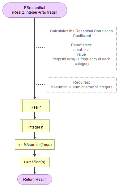
It takes as input the z-value and an array of integers with the observed frequencies.
It uses the function a small helper function to determine the sum of an array.
Flowgorithm file: FL-ESrosenthal.fprg.
with Python
Jupyter Notebook: ES - Rosenthal Correlation.ipynb
with R (studio)
video to be uploaded
R script: ES - Rosenthal Correlation (one-sample).R
Data file: GSS2012a.csv.
with SPSS
Data file: GSS2012-Adjusted.sav
with an online calculator
Enter the standardized test statistic, and the sample size:
manually (Formula and Example)
Formula
The formula to determine the Rosenthal Correlation Coefficient is:
\(r_{Rosenthal}=\frac{Z}{\sqrt{n}}\)
In this formula Z is the Z-statistic, which in the case of a Wilcoxon one-sample test is the adjusted W statistic, and n the sample size.
Example
Note this is a different example than used in this section.
We are given six scores from an ordinal scale and like to test if the median is significantly different from 3. The six scores are:
\(x=\left(4,4,5,1,5,3 \right )\)
In the previous section we already calculated the adjusted W statistic, so we can set:
\(Z=W_*=\frac{\sqrt{210}}{15}\approx0.966\)
Since there are six scores we also know:
\(n=6\)
Filling out the formula for the Rosenthal Correlation, we then get:
\(r_{Rosenthal}=\frac{Z}{\sqrt{n}}=\frac{\frac{\sqrt{210}}{15}}{\sqrt{6}}=\frac{\sqrt{210}}{15\times\sqrt{6}}=\frac{1}{15}\times\frac{\sqrt{210}}{\sqrt{6}}\)
\(=\frac{1}{15}\times\sqrt{\frac{210}{6}}=\frac{1}{15}\times\sqrt{35}=\frac{1}{15}\sqrt{35}\approx0.3944\)
Let's finish by combining all the reports parts now in the next part.
Alternative effect size measures can also be a (matched pair) rank-biserial correlation coefficient (see for example King and Minium (2008, p. 403).
Click here to see how you can obtain the (matched pair) Rank Biserial Coefficient One-Sample...
with Excel
Excel file used in video: ES - Rank Biserial.xlsm
with Flowgorithm
A flowgorithm for the (matched pair) Rank Biserial Coefficient One-Sample in Figure 1.
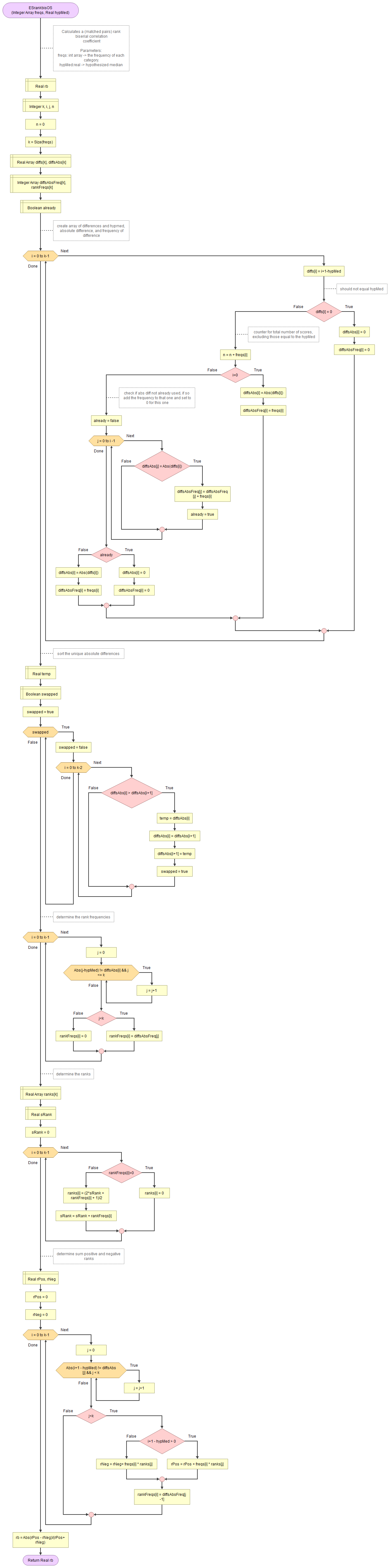
It takes as an array of integers with the observed frequencies and the hypothesized median.
Flowgorithm file: FL-ESrankbisOS.fprg.
with Python
video to be uploaded
Jupyter notebook: ES - Rank Biserial Coefficient.ipynb
Data file: GSS2012a.csv.
with R (studio)
video to be uploaded
Jupyter notebook: ES - Rank Biserial Coefficient (one-sample).ipynb
R script: ES - Rank Biserial Coefficient (one-sample).R
Data file: GSS2012a.csv.
with SPSS
Data file: GSS2012-Adjusted.sav
manually (Formula and Example)
Formula
The formula to determine the Matched Pairs Rank-Biserial Coefficient is:
\( r_{rb} = \frac{4\times\left|T-\left(\frac{R_{+} + R_{-}}{2}\right)\right|}{n\times\left(n+1\right)} \)
In this formula \(R_{+}\) is the sum of the positive ranks, \(R_{-}\) the sum of the negative ranks, \(T\) the smaller of the two, i.e. \(min\left(R_+, R_-\right)\), and \(n\), the number of ranks.
The formula can actually be re-written to (Kerby, 2014, p. 5)
\( r_{rb} = \frac{\left|R_{+} - R_{-}\right|}{R} \)
with \(R = R_{+} + R_{-}\)
Proof for the equivelance of the two formulas
The first formula is:
\( r_{rb} = \frac{4\times\left|T-\left(\frac{R_{+} + R_{-}}{2}\right)\right|}{n\times\left(n+1\right)} \)
If we assume \(T = R_{+}\) we can substitute this:
\( = \frac{4\times\left|R_{+}-\left(\frac{R_{+} + R_{-}}{2}\right)\right|}{n\times\left(n+1\right)} \)
\( = \frac{\left|4\times R_{+}-\left(4\times\frac{R_{+} + R_{-}}{2}\right)\right|}{n\times\left(n+1\right)} \)
\( = \frac{\left|4\times R_{+}-2\times\left(R_{+} + R_{-}\right)\right|}{n\times\left(n+1\right)} \)
\( = \frac{\left|2\times R_{+}-2\times R_{-}\right|}{n\times\left(n+1\right)} \)
\( = \frac{2\times\left|\left(R_{+}-R_{-}\right)\right|}{n\times\left(n+1\right)} \)
If we had used \(T = R_{-}\) instead, we also would have ended with the step above. This will be shown after we finish with assuming \(T = R_{+}\)
\( = \frac{2}{n\times\left(n+1\right)} \times \left|\left(R_{+}-R_{-}\right)\right| \)
\( = \frac{1}{\frac{n\times\left(n+1\right)}{2}} \times \left|\left(R_{+}-R_{-}\right)\right| \)
Now use that \(R\) is the sum of all ranks. The sum of the ranks is simply adding them all up. This would be 1 + 2 + ... + n. This can be calculated quickly using:
\( R = \sum \text{ranks} = \frac{n\times\left(n+1\right)}{2} \)
\( = \frac{1}{R} \times \left|\left(R_{+}-R_{-}\right)\right| \)
\( = \frac{\left|\left(R_{+}-R_{-}\right)\right|}{R} \)
If we had assumed \(T = R_{-}\) we had started with:
\( = \frac{4\times\left|R_{-}-\left(\frac{R_{+} + R_{-}}{2}\right)\right|}{n\times\left(n+1\right)} \)
\( = \frac{\left|4\times R_{-}-\left(4\times\frac{R_{+} + R_{-}}{2}\right)\right|}{n\times\left(n+1\right)} \)
\( = \frac{\left|4\times R_{-}-2\times\left(R_{+} + R_{-}\right)\right|}{n\times\left(n+1\right)} \)
\( = \frac{\left|-2\times R_{+}-2\times R_{-}\right|}{n\times\left(n+1\right)} \)
\( = \frac{2\times\left|\left(R_{+}-R_{-}\right)\right|}{n\times\left(n+1\right)} \)
Which we also saw earlier when assuming \(T = R_{+}\), hence Q.E.D.
Example
We are given six scores from an ordinal scale and like to test if the median is significantly different from 3. The six scores are:
\( x=\left(4,4,5,1,5,3\right) \)
The hypothesized median was given to be 3, so:
\( \theta=3 \)
First we now remove any score from x that is equal to the hypothesized median, which in the example is only the last score. So we set:
\( y=\left(4,4,5,1,5\right) \)
Then we determine the difference with the hypothesized median:
\( d=\left(4-3,4-3,5-3,1-3,5-3\right)=\left(1,1,2,-2,2\right) \)
To determine the ranks, we need tha absolute values of these:
\( |d|=\left(|1|,|1|,|2|,|-2|,|2|\right)=\left(1,1,2,2,2\right) \)
Then we rank these absolute differences. The lowest score is a 1, but this occurs twice. So they take up rank 1 and 2, or on average rank 1.5. Then we have a score of 2, but this occurs three times. So they take ranks 3, 4 and 5, or on average rank 4. It is these average ranks that we need:
\( r=\left(1.5,1.5,4,4,4\right) \)
To determine \(R^{+}\) we sum up the ranks, but only for those that had a positive deviation (from d). The fourth entry in d is negative (-2), so we do not add the rank of 4 from that score. We therefor get:
\( R^{+}=1.5+1.5+4+4=11 \)
To determine \(R^{-}\) we sum up the ranks, but only for those that had a negative deviation (from d). The fourth entry in d is the only one negative (-2). We therefor get:
\( R^{-}=4 \)
\( T\) is the minimum of the two, which in this case is 4. The number of ranks we have is 5, so we can finally fill out the formula:
\( r_{rb} = \frac{4\times\left|4-\left(\frac{11 +4}{2}\right)\right|}{5\times\left(5+1\right)} \)
\( = \frac{4\times\left|4-\left(\frac{15}{2}\right)\right|}{5\times6} \)
\( = \frac{4\times\left|-3.5\right|}{30} \approx 0.4667\)
Using the alternative faster formula, with \( R = 4+11 = 15\):
\( r_{rb} = \frac{\left|11 - 4\right|}{15} = \frac{7}{15} \approx 0.4667 \)
If you used a sign-test, there is no z-value to be used in the correlation coefficient. Mangiafico (2016) suggests to use a dominance score, or a value similar to Vargha-Delaney's A.
Single ordinal variable
![]()

Google adds