Wilcoxon Signed Rank Distribution

Click here for a video explaining the concept

The Wilcoxon signed rank distribution shows how many different options there are to obtain a sum of ranks. For example if we have 5 unique scores, there are three ways to obtain a sum of ranks of 6:

a rank of 1, 2 and 3
a rank of 1 and 5
a rank of 2 and 3

The distribution is based on counts, and is therefor a so-called discrete distribution (there are no 'in between' values (e.g. 3.15). It is however symmetrical.

The counts for each possible sum of ranks are usually converted to probabilities. This is simply done by dividing the count by the sum of all counts, and results in the probability mass distribution. If we keep adding these probabilities we get the cumulative density distribution.

If we had a sample size of 5 and wanted to know the p-value for a two-sided test that had a sum of ranks of 6, we could look at the probability mass distribution as shown in Figure 1.

Figure 1
Wilcoxon Signed Rank Distribution n=5

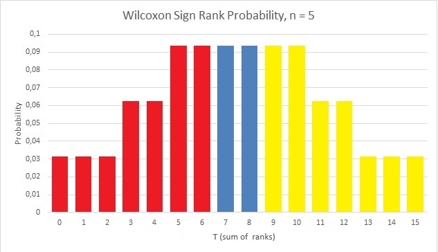
We should add all the red-bars, since we are interested in a score of 6 or even more extreme (rare). This would be also the result of a cumulative density function (cdf) on this distribution. But, equally rare would be the values on the other side of the symmetry, the ones highlighted in yellow, so we should also add those. However, since the distribution is symmetrical, the sum of the red bars, would be the same as the sum of the yellow bars, so we can simply double the cdf result.

The distribution will start to look a lot like a normal distribution when the sample size gets larger. The distribution is shown in Figure 2 for a few different sample sizes.

Figure 2
Cumulative Wilcoxon Signed Rank Distribution Example for Various n

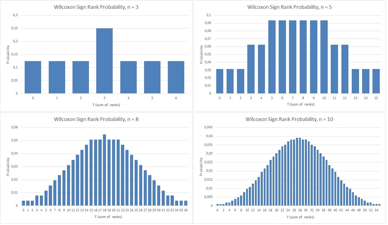
Already at n=10 the figure starts to look very similar to a normal distribution, which is why for large values of n, the normal approximation is often used.

Note that this distribution is used for an exact Wilcoxon signed rank test, either as a one-sample, or a paired sample. There is also a (Mann-Whitney-) Wilcoxon Rank Sum distribution, which is used for a Mann-Whitney U test which is equal to a Wilcoxon rank sum test. The test-statistic for those using the signed rank distribution is usually \(T\), while for the rank-sum it is \(W\) or \(U\).

There are different ways to get the distribution, which are explained in the sections below.

Use some software (easy)

Excel

The Excel file used in the videos can be downloaded here.

with stikpetE add-in

Using enumeration.

Using Recursive Formula.

Using Shift Algorithm

Python

The notebook used in the videos can be downloaded here.

with stikpetP library

Using enumeration.

Using Recursive Formula.

Using Shift Algorithm

The notebook used in the videos can be downloaded here.

with stikpetR library

Using enumeration.

Using Recursive Formula.

Using Shift Algorithm

Using SignRank

Use tables (old school)

Before computers we often made use of tables, like the one shown in figure 1.

Figure 1, 2, and 3
Cumulative Wilcoxon Signed Rank Distribution Table

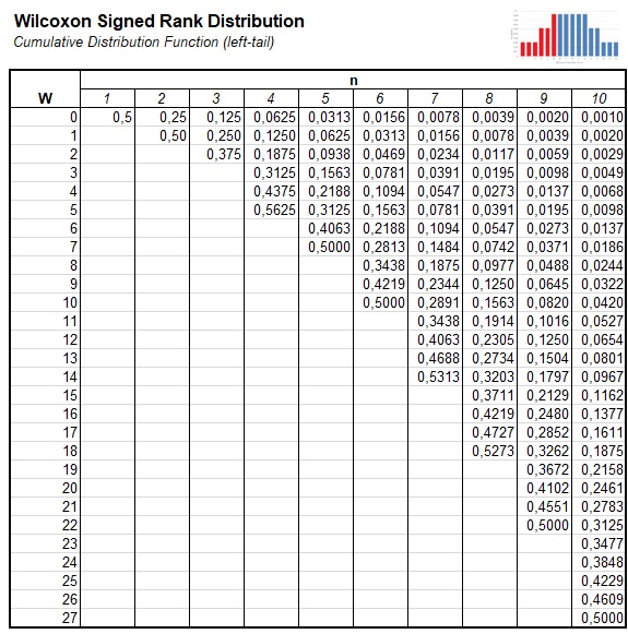
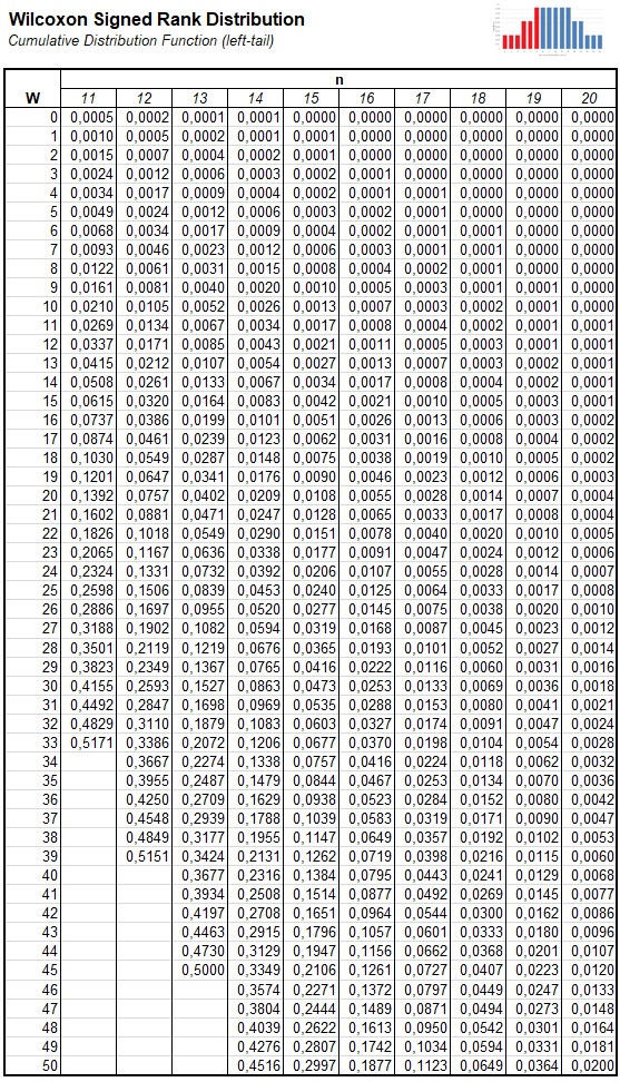
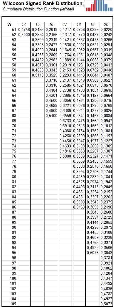
To illustrate how to use this, let's say we had a sum of ranks of 6, i.e. \(T=6\) and a sample size ( (\n\) ) of 5. We then look for the intersection of the row where \(T=6\) and the column of \(n=5\) as illustrated in figure 4

Figure 4
Cumulative Wilcoxon Signed Rank Distribution Table Example

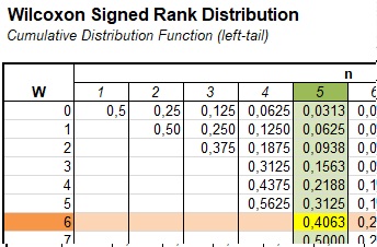
The highlighted cell in yellow has a value of 0.4063. This indicates that the probability of a sum of ranks of 6 or less, if the sample size is 5 is 0.4063 (41%). We often want the two-sided p-value, so we can simply double this, since the distribution is symmetrical: \(2\times0.4063 = 0.8126\).

You might notice the table ends for each sample size, once it hits 0.5 or more. This is because the distribution is symmetrical. If we have a sample size of 6, the sum of all ranks would be \(\sum_{i=1}^6 i = \frac{6\times \left(6 + 1\right)}{2} = \binom{6+1}{2} = 21\). If we have a T value of 16, we can look at T of 21 - 16 = 5, and then subtract the result from 1.

A table similar as the one shown in Figure 1, 2 and 3 can be found for example in Wilcoxon et al. (1970, pp. 237-259).

An alternative type of table shows critical values, as shown in figure 5.

Figure 5
Cumulative Wilcoxon Signed Rank Distribution Critical Values Table

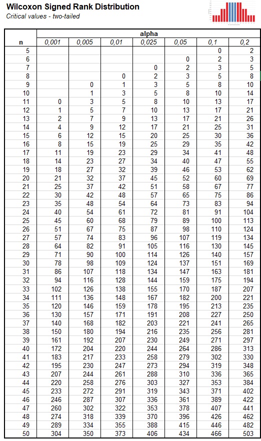
If we have a sample size of 12, we can find that the critical T value for a two sided test with alpha set at 0.05 would be 13. We would need a T value of 13 or less. Alternatively we can look at the sum of all ranks with 12 cases: \(\sum_{i=1}^{12} i = 78\) and therefor a T of (78-13=) 65 or more would also work.

Note that for samples sizes of 4 or less, none of the alpha levels will be possible to reach, while for sample sizes of more than 50 a normal approximation is usually used.

Do the math (hard core)

Listing All Options

To illustrate how we can create the distribution manually we go over a few different possible sample sizes.

If we only have one score in the sample, we then also only have one rank. It could either be for a score above the hypothesized score or below. So using a 1 for above and a 0 for below, e have either

rank	1	2
1	0	1
rank sum	0	1

If we only have two ranks, we copy the table of the first one, copy it again and paste it next to it, add one row and fill half with zeros and the other half with ones:

rank	1	2	3	4
1	0	1	0	1
2	0	0	1	1
rank sum	0	1	2	3

Repeat for three ranks:

rank	1	2	3	4	5	6	7	8
1	0	1	0	1	0	1	0	1
2	0	0	1	1	0	0	1	1
3	0	0	0	0	1	1	1	1
rank sum	0	1	2	3	3	4	5	6

The rank sum is calculated by summing the ranks for which there is a 1. For example in the above table for option 6 we have 1 time rank 1, 0 times rank 2 and 1 time rank 3, so \(1\times 1 + 0 \times 2 + 1\times 3 = 4\).

For four ranks:

rank	1	2	3	4	5	6	7	8	9	10	11	12	13	14	15	16
1	0	1	0	1	0	1	0	1	0	1	0	1	0	1	0	1
2	0	0	1	1	0	0	1	1	0	0	1	1	0	0	1	1
3	0	0	0	0	1	1	1	1	0	0	0	0	1	1	1	1
4	0	0	0	0	0	0	0	0	1	1	1	1	1	1	1	1
rank sum	0	1	2	3	3	4	5	6	4	5	6	7	7	8	9	10

One more with five ranks:

rank	1	2	3	4	5	6	7	8	9	10	11	12	13	14	15	16	17	18	19	20	21	22	23	24	25	26	27	28	29	30	31	32
1	0	1	0	1	0	1	0	1	0	1	0	1	0	1	0	1	0	1	0	1	0	1	0	1	0	1	0	1	0	1	0	1
2	0	0	1	1	0	0	1	1	0	0	1	1	0	0	1	1	0	0	1	1	0	0	1	1	0	0	1	1	0	0	1	1
3	0	0	0	0	1	1	1	1	0	0	0	0	1	1	1	1	0	0	0	0	1	1	1	1	0	0	0	0	1	1	1	1
4	0	0	0	0	0	0	0	0	1	1	1	1	1	1	1	1	0	0	0	0	0	0	0	0	1	1	1	1	1	1	1	1
5	0	0	0	0	0	0	0	0	0	0	0	0	0	0	0	0	1	1	1	1	1	1	1	1	1	1	1	1	1	1	1	1
rank sum	0	1	2	3	3	4	5	6	4	5	6	7	7	8	9	10	5	6	7	8	8	9	10	11	9	10	11	12	12	13	14	15

Next we look at how often each rank sum actually occurs. Note that the minimum is of course 0, and the maximum would be the sum of all ranks, for 1 to n, in math notation \(\sum_{i=1}^n i = \frac{n\times \left(n + 1\right)}{2} = \binom{n+1}{2}\).

We also take this count (frequency) and divide it by the total number of counts we have, which should be equal to \(2^n\). This is the probability mass distribution. If we keep adding these up we also get the cumulative probability distribution.

For n = 1 it is fairly simple:

rank sum	freq.	prob.	cumul. prob.
0	1	1/2 = 0.5	1/2 = 0.5
1	1	1/2	2/2 = 1

For n = 2, we have \(2^2 = 4\) variations, and the rank sum has a maximum of \(\sum_{i=1}^2 i = \frac{2\times \left(2 + 1\right)}{2} = \binom{2+1}{2}\) = 3:

rank sum	freq.	prob.	cumul. prob.
0	1	1/4	1/4
1	1	1/4 = 0.25	2/4 = 1/2 = 0.5
2	1	1/4 = 0.25	3/4 = 0.75
3	1	1/4 = 0.25	4/4 = 1

For n = 3, we have \(2^3 = 8\) variations, and the rank sum has a maximum of \(\sum_{i=1}^3 i = \frac{3\times \left(3 + 1\right)}{2} = \binom{3+1}{2}\) = 6:

rank sum	freq.	prob.	cumul. prob.
0	1	1/8 = 0.125	1/8
1	1	1/8 = 0.125	2/8 = 1/4 = 0.25
2	1	1/8 = 0.125	3/8 = 0.375
3	2	2/8 = 1/4 = 0.25	5/8 = 0.625
4	1	1/8 = 0.125	6/8 = 3/4 = 0.75
5	1	1/8 = 0.125	7/8 = 0.875
6	1	1/8 = 0.125	8/8 = 1

For n = 4, we have \(2^4 = 16\) variations, and the rank sum has a maximum of \(\sum_{i=1}^4 i = \frac{4\times \left(4 + 1\right)}{2} = \binom{4+1}{2}\) = 10:

rank sum	freq.	prob.	cumul. prob.
0	1	1/16 = 0.625	1/16 = 0.625
1	1	1/16 = 0.625	2/16 = 1/8 = 0.125
2	1	1/16 = 0.625	3/16 = 0.1875
3	2	2/16 = 1/8 = 0.125	5/16 = 0.3125
4	2	2/16 = 1/8 = 0.125	7/16 = 0.4375
5	2	2/16 = 1/8 = 0.125	9/16 = 0.5625
6	2	2/16 = 1/8 = 0.125	11/16 = 0.6875
7	2	2/16 = 1/8 = 0.125	13/16 = 0.8125
8	1	1/16 = 0.625	14/16 = 7/8 = 0.875
9	1	1/16 = 0.625	15/16 = 0.9375
10	1	1/16 = 0.625	16/16 = 1

For n = 5, we have \(2^5 = 32\) variations, and the rank sum has a maximum of \(\sum_{i=1}^5 i = \frac{5\times \left(5 + 1\right)}{2} = \binom{5+1}{2}\) = 32:

rank sum	freq.	prob.	cumul. prob.
0	1	1/32 = 0.03125	1/32 = 0.03125
1	1	1/32 = 0.03125	2/32 = 1/16 = 0.0625
2	1	1/32 = 0.03125	3/32 = 0.09375
3	2	2/32 = 1/16 = 0.0625	5/32 = 0.15625
4	2	2/32 = 1/16 = 0.0625	7/32 = 0.21875
5	3	3/32	10/32 = 5/16 = 0.3125
6	3	3/32	13/32 = 0.40625
7	3	3/32	16/32 = 1/2 = 0.5
8	3	3/32	19/32 = 0.59375
9	3	3/32	22/32 = 11/16 = 0.6875
10	3	3/32	25/32 = 0.78125
11	2	2/32 = 1/16 = 0.0625	27/32 = 0.84375
12	2	2/32 = 1/16 = 0.0625	29/32 = 0.90625
13	1	1/32 = 0.03125	30/32 = 15/16 = 0.9375
14	1	1/32 = 0.03125	31/32 = 0.96875
15	1	1/32 = 0.03125	32/32 = 1

Using Recursive Formula

Instead of creating the table and calculating the probabilities, there is a recursive formula to calculate the frequencies (McCornack, 1965, p. 864):

\(srf\left(x,y\right)=\begin{cases} 0 & x \lt 0 \\ 0 & x\gt\binom{y+1}{2} \\ 1 & y=1 \wedge \left( x=0\vee x=1 \right) \\ srf^*\left(x,y\right) & y\geq 0 \end{cases} \)

with:

\(srf^*\left(x,y\right) = srf\left(x-y,y-1\right) + srf\left(x,y-1\right) \)

The probability mass function (pmf) is then simply:

\(wpmf\left(x, n\right) = \frac{srf\left(x,n\right)}{2^n}\)

The cumulative density function is to simply sum up the pmf's:

\(wcdf\left(T, n\right) = \sum_{i=0}^T wpmf\left(i, n\right)\)

Let's say we wanted to know the freq. if we have 5 ranks for a rank sum of 6. So \(srf\left(6,5\right)\). 6 is not less than 0, and it is also not greater than \(\binom{5 + 1}{2} = 15\), so we use \(srf^*\)

Figure 1 shows all the steps we need to make using the srf formula.

Figure 1
srf example for 6,5 part 1

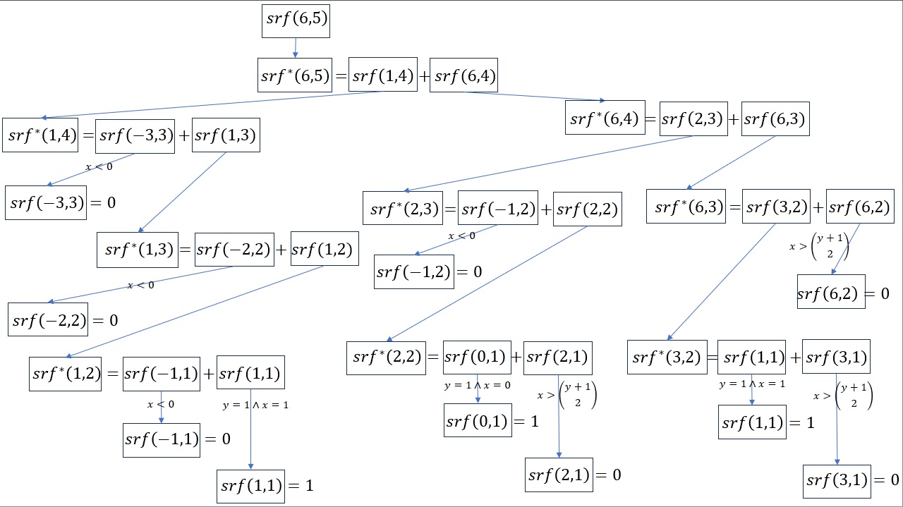
Once all the steps are done, we can backtrace everything as shown in Figure 2.

Figure 2
srf example for 6,5 part 2

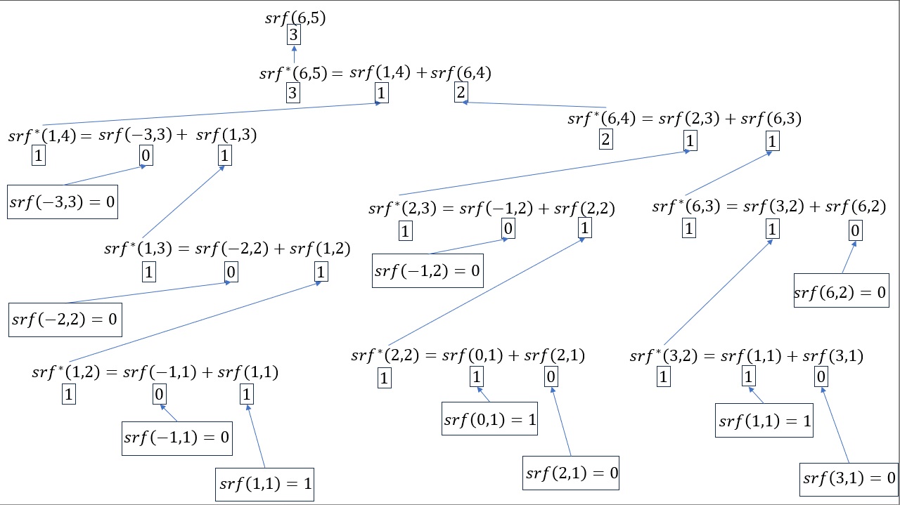
Once we know the frequencies using the srf function, it is fairly easy to determine the probability:

\(wpmf\left(6, 5\right) = \frac{srf\left(6,5\right)}{2^5} = \frac{3}{32} = 0.09375\)

Using shift-algorithm

Another approach is the shift-algorithm from Streitberg and Röhmel (1987), and can also be found in Munzel and Brunner (2002). This works as follows.

Start with listing all values from 0 to the maximum possible sum of ranks (\(T_{max}\)), so 0 to \(\frac{n\times\left(n+1\right)}{2}\).
Create a vector with the value 1 followed by \(T_{max}\) times a 0.
Create a shifted vector by moving all values by 1.
Add the two results (the original and the shifted version)
This will be the updated vector
Shift the vector now by 2
Add the two results (the updated vector with and the two shifted version)
Repeat these steps each time shifting by one more than the previous. Stop when n-times shifting has been done.

The animated gif in Figure 3, shows the steps for n=5.

Figure 3
shift-Algorithm for Wilcoxon sign distribution Example

The last step provides the entire frequency distribution. From this the probability density and cumulative density can easily be obtained.

The sum of all the frequencies should always be \(2^n\), in the example where n=5 we have \(2^5 = 32\). The frequency for a rank sum of 6 is 3, so the probability is simply \(\frac{3}{32}\). For the cdf we can can simply sum all the results up to and including 6 to get \(1+1+1+2+2+3+3 = 13\), and divide this again by the total sum of all frequencies to get the cumulative probability of \(\frac{13}{32} = 0.40625\).

Other Algorithms

There are more algorithms, which might be better/faster. For example:

The split-up algorithm from Van de Wiel (2001)
Fourier method from Pagano and Tritchler (1983)
Network algorithm from Mehta et. al. (1988)
Algorithm from Yeo (2017)

Distributions

Google adds