
Cohen d
Introduction
Cohen d is an effect size measure, that compares the difference between two means. It informs on how many standard deviations the difference is. There are four variations of this effect size measure:
- \(d'\), is the version that compares the sample mean with the mean according to the null hypothesis (i.e. the mean expected in the population)
- \(d_s\), is the version that compares the sample mean of two independent groups (independent samples) and is the same as Hedges g
- \(d_z\), is the vesion that compares the sample mean of paired samples
- \(d\), is used to compare the maximum and minimum sample mean of multiple groups
Obtaining the Measure
Click here to see how to obtain Cohen d' for a one-sample test.
with Flowgorithm
A flowgorithm for Cohen's d (one-sample) in Figure 1.
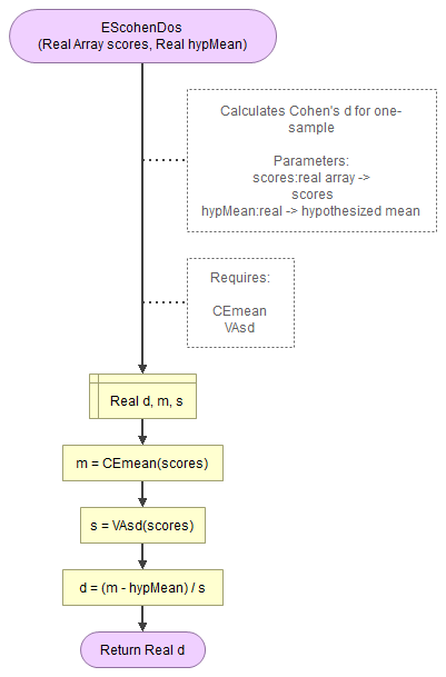
It takes as input paramaters the scores and the hypothesized mean.
It uses a function for the mean (CEmean), standard deviation (VAsd) which in turn use the MAsumReal function (sums array or real values).
Flowgorithm file: FL-EScohenDos.fprg.
with Python
Jupyter Notebook used in video: ES - Cohen d (one-sample) (P).ipynb.
with stikpetP
without stikpetP library
with R (Studio)
Jupyter Notebook used in video: ES - Cohen d (one-sample) (R).ipynb.
with stikpetR
without stikpetR library
with SPSS
This has become available in SPSS 27. As mentioned on this site, there is no option in earlier versions of SPSS to determine Cohen's D, but it can easily be calculated using by using the output from the t-test and entering the results below in the 'Online calculator' option, or using the 'Compute variable' option as shown in the video.
SPSS 27 or later
Datafile used in video: GSS2012-Adjusted.sav
SPSS 26 or earlier
Datafile used in video: GSS2012-Adjusted.sav
with an online calculator
Enter the sample mean, the hypothesized population mean, and the sample standard deviation:
manually (formula and example)
Formula's
The formula for Cohen's d for a one-sample t-test is:
\(d'=\frac{\bar{x}-\mu_{H_{0}}}{s}\)
Where x̄ is the sample mean, μH0 the expected mean in the population (the mean according to the null hypothesis), and s the sample standard deviation.
The formula for the sample standard deviation is:
\(s=\sqrt{\frac{\sum_{i=1}^{n}\left(x_{i}-\bar{x}\right)^{2}}{n-1}}\)
In this formula xi is the i-th score, x̄ is the sample mean, and n is the sample size.
The sample mean can be calculated using:
\(\bar{x}=\frac{\sum_{i=1}^{n}x_{i}}{n}\)
Example (different example)
We are given the ages of five students, and have an hypothesized population mean of 24. The ages of the students are:
\(X=\left\{18,21,22,19,25\right\}\)
Since there are five students, we can also set n = 5, and the hypothesized population of 24 gives \(\mu_{H_{0}}=24\)
For the standard deviation, we first need to determine the sample mean:
\(\bar{x}=\frac{\sum_{i=1}^{n}x_{i}}{n}=\frac{\sum_{i=1}^{5}x_{i}}{5}=\frac{18+21+22+19+25}{5}\)
\(=\frac{105}{5}=21\)
Then we can determine the standard deviation:
\(s=\sqrt{\frac{\sum_{i=1}^{n}\left(x_{i}-\bar{x}\right)^{2}}{n-1}}=\sqrt{\frac{\sum_{i=1}^{5}\left(x_{i}-21\right)^{2}}{5-1}}=\sqrt{\frac{\sum_{i=1}^{5}\left(x_{i}-21\right)^{2}}{4}}\)
\(=\sqrt{\frac{\left(18-21\right)^{2}}{4}+\frac{\left(21-21\right)^{2}}{4}+\frac{\left(22-21\right)^{2}}{4}+\frac{\left(19-21\right)^{2}}{4}+\frac{\left(25-21\right)^{2}}{4}}\)
\(=\sqrt{\frac{\left(-3\right)^{2}}{4}+\frac{\left(0\right)^{2}}{4}+\frac{\left(1\right)^{2}}{4}+\frac{\left(-2\right)^{2}}{4}+\frac{\left(4\right)^{2}}{4}}\)
\(=\sqrt{\frac{9}{4}+\frac{0}{4}+\frac{1}{4}+\frac{4}{4}+\frac{16}{4}}=\sqrt{\frac{9+0+1+4+16}{4}}=\sqrt{\frac{30}{4}}\)
\(=\sqrt{\frac{15}{2}}=\frac{1}{2}\sqrt{15\times2}=\frac{1}{2}\sqrt{30}\approx2.74\)
Now for Cohen's d:
\(d=\frac{\bar{x}-\mu_{H_{0}}}{s}=\frac{21-24}{\frac{1}{2}\sqrt{30}}=\frac{-3}{\frac{\sqrt{30}}{2}}\)
\(=\frac{-3\times2}{\sqrt{30}}=\frac{-6}{\sqrt{30}}=\frac{-6}{\sqrt{30}}\times\frac{\sqrt{30}}{\sqrt{30}}=\frac{-6\times\sqrt{30}}{\sqrt{30}\times\sqrt{30}}\)
\(=\frac{-6\times\sqrt{30}}{30}=\frac{-6}{30}\times\sqrt{30}=-\frac{1}{5}\sqrt{30}\approx1.0954\)
Click here to see how to obtain Cohen ds for independent samples.
with Excel
Excel file: ES - Cohen d and Hedges g (ind samples) (E).xlsm
with stikpetE
To Be Made
without stikpetE
To Be Made
with Python
Jupyter Notebook: ES - Cohen d and Hedges g (ind samples) (P).ipynb
with stikpetP
To Be Made
without stikpetP
with R (studio)
Jupyter Notebook: ES - Cohen d and Hedges g (ind samples) (R).ipynb
with stikpetR
To Be Made
without stikpetR
with SPSS
version 27+
versions prior to 27
Unfortunately versions prior to 27 do not have an option in the GUI to determine Cohen's d. However you can either use the output from the independent samples t-test and enter the results in the online calculator (see below), or use SPSS syntax. The video will show each option
Online calculator
Enter the requested information below:
Manually
Cohen's ds formula is:
\(d_{s}=\frac{\bar{x}_{1}-\bar{x}_{1}}{s_{pooled}}\)
In this formula \(\bar{x}_{i}\) is the mean for category i, which can be calculated by:
\(\bar{x}_{i}=\frac{\sum_{j=1}^{n_{i}}x_{i,j}}{n_{i}}\)
In this formula xi,j is the j-th score in category i, and ni is the number of cases in category i
spooled is the pooled standard deviation. In formula notation this is:
\(s_{pooled}=\sqrt\frac{SS_{1}+SS_{2}}{N-2}\)
In this formula N is the total number of cases (combination of both categories), and SSi the sum of squared differences with the mean, which in formula notation is:
\(SS_{i}=\sum_{j=1}^{n_{i}}\left(x_{i,j}-\bar{x}_i\right)^{2}\)
An example.
Note: a different example than the one used in the rest of this section, to keep calculations a bit shorter.
Given are the scores of males (category 1) and females (category 2):
\(X_{1}=\left(8,3,2,1,1\right)\)
\(X_{2}=\left(7,7,5,3,9,8\right)\)
The first category, has 5 scores, so n1 = 5, and for the second category we have n2 = 6. Let's begin with determining the mean per category:
\(\bar{x}_{1}=\frac{\sum_{j=1}^{n_{1}}x_{1,j}}{n_{1}}=\frac{\sum_{j=1}^{5}x_{1,j}}{5}=\frac{8+3+2+1+1}{5}=\frac{15}{5}=3\)
\(\bar{x}_{2}=\frac{\sum_{j=1}^{n_{2}}x_{2,j}}{n_{2}}=\frac{\sum_{j=1}^{6}x_{2,j}}{6}=\frac{7+7+5+3+9+8}{6}=\frac{39}{6}=\frac{13}{2}=6.5\)
Then we can determine the sum of squares per category. First the male category:
\(SS_{1}=\sum_{j=1}^{n_{1}}\left(x_{1,j}-\bar{x}_1\right)^{2}=\sum_{j=1}^{5}\left(x_{1,j}-3\right)^{2}\)
\(=\left(8-3\right)^{2}+\left(3-3\right)^{2}+\left(2-3\right)^{2}+\left(1-3\right)^{2}+\left(1-3\right)^{2}\)
\(=\left(5\right)^{2}+\left(0\right)^{2}+\left(-1\right)^{2}+\left(-2\right)^{2}+\left(-2\right)^{2}=25+0+1+4+4=34\)
And for the female category:
\(SS_2=\sum_{j=1}^{n_2}\left(x_{2,j}-\bar{x}_2\right)^{2}=\sum_{j=1}^{6}\left(x_{2,j}-\frac{13}{2}\right)^{2}\)
\(=\left(7-\frac{13}{2}\right)^{2}+\left(7-\frac{13}{2}\right)^{2}+\left(5-\frac{13}{2}\right)^{2}+\left(3-\frac{13}{2}\right)^{2}+\left(9-\frac{13}{2}\right)^{2}+\left(8-\frac{13}{2}\right)^{2}\)
\(=\left(\frac{14}{2}-\frac{13}{2}\right)^{2}+\left(\frac{14}{2}-\frac{13}{2}\right)^{2}+\left(\frac{10}{2}-\frac{13}{2}\right)^{2}+\left(\frac{6}{2}-\frac{13}{2}\right)^{2}+\left(\frac{18}{2}-\frac{13}{2}\right)^{2}+\left(\frac{16}{2}-\frac{13}{2}\right)^{2}\)
\(=\left(\frac{14-13}{2}\right)^{2}+\left(\frac{14-13}{2}\right)^{2}+\left(\frac{10-13}{2}\right)^{2}+\left(\frac{6-13}{2}\right)^{2}+\left(\frac{18-13}{2}\right)^{2}+\left(\frac{16-13}{2}\right)^{2}"\)
\(=\left(\frac{1}{2}\right)^{2}+\left(\frac{1}{2}\right)^{2}+\left(\frac{-3}{2}\right)^{2}+\left(\frac{-7}{2}\right)^{2}+\left(\frac{5}{2}\right)^{2}+\left(\frac{3}{2}\right)^{2}\)
\(=\frac{1}{4}+\frac{1}{4}+\frac{9}{4}+\frac{49}{4}+\frac{25}{4}+\frac{9}{4}=\frac{1+1+9+49+25+9}{4}\)
\(=\frac{94}{4}=\frac{47}{2}=23.5\)
The pooled standard deviation therefor is:
\(s_{pooled}=\sqrt\frac{SS_{1}+SS_{2}}{N-2}=\sqrt\frac{34+\frac{47}{2}}{11-2}\)
\(=\sqrt\frac{\frac{68}{2}+\frac{47}{2}}{9}=\sqrt\frac{\frac{68+47}{2}}{9}=\sqrt\frac{\frac{115}{2}}{9}=\sqrt\frac{115}{2\times9}\)
\(=\sqrt\frac{115}{18}=\frac{1}{18}\sqrt{115\times18}=\frac{1}{18}\sqrt{115\times2\times9}=\frac{3}{18}\sqrt{115\times2}\)
And finally Cohen's ds:\(=\frac{3}{18}\sqrt{115\times2}=\frac{1}{6}\sqrt{230}\approx2.53\)
\(d_s=\frac{\bar{x}_{1}-\bar{x}_{1}}{s_{pooled}}=\frac{3-\frac{13}{2}}{\frac{1}{6}\sqrt{230}}=\frac{\frac{6}{2}-\frac{13}{2}}{\frac{1}{6}\sqrt{230}}=\frac{\frac{6-13}{2}}{\frac{\sqrt{230}}{6}}\)
\(=\frac{\frac{6-13}{2}}{\frac{\sqrt{230}}{6}}=\frac{\frac{-7}{2}}{\frac{\sqrt{230}}{6}}=\frac{-7\times6}{2\times\sqrt{230}}=\frac{-7\times3}{\sqrt{230}}=\frac{-21}{\sqrt{230}}\)
\(=\frac{-21\times\sqrt{230}}{230}=-\frac{21}{230}\times\sqrt{230}\approx-1.38\)
Click here to see how to obtain Cohen dz for paired samples.
with Python
with R (studio)
with SPSS
version 27+
versions prior to 27
Manually
Formulas
\(d_z=\frac{\bar{d}}{s_d}=\frac{t}{\sqrt{n}}\)
\(g=d_z\times{J(df)}\)
\(J(df)=\frac{\Gamma{\left(\frac{df}{2}\right)}}{\sqrt{\frac{df}{2}}\times\Gamma\left(\frac{df-1}{2}\right)}\approx1-\frac{3}{4\times{df}-1}\)
See the manually part in the test section for the formulas for \(\bar{d},s_d,t,df\)
Example
Note: continuation of the example in the manually part of the test section.
We are given the following pairs:
\(P=\left\{(9,8),(2,),(5,3),(4,6),(8,4),(8,3)\right\}\)
Since the second pair is missing a score, it will not be used and removed, so:
\(X=\left\{(9,8),(5,3),(4,6),(8,4),(8,3)\right\}\)
There are five pairs remaining, so n = 5.
In the test section we already calculated the following:
\(\bar{d}=2,s_d=\frac{\sqrt{30}}{2},t=\frac{2\sqrt{6}}{3},df=4\)
Cohen's d is therefor:
\(d_z=\frac{\bar{d}}{s_d}=\frac{2}{\frac{\sqrt{30}}{2}}=\frac{2\times2}{\sqrt{30}}=\frac{4\times\sqrt{30}}{\sqrt{30}\times\sqrt{30}}\)
\(=\frac{4\times\sqrt{30}}{30}=\frac{2\sqrt{30}}{15}\approx0.7303\)
If we had used the alternative formula, we would have gotten the same result:
\(d_z=\frac{t}{\sqrt{n}}=\frac{\frac{2\sqrt{6}}{3}}{\sqrt{5}}=\frac{2\sqrt{6}}{3\times\sqrt{5}}=\frac{2\sqrt{6}\times\sqrt{5}}{3\times\sqrt{5}\times\sqrt{5}}\)
\(=\frac{2\sqrt{6\times5}}{3\times5}=\frac{2\sqrt{30}}{15}\approx0.7303\)
For the Hedges correction we can use the approximation. That would yield:
\(J(df)\approx1-\frac{3}{4\times{df}-1}=1-\frac{3}{4\times{4}-1}=1-\frac{3}{15}=1-\frac{1}{5}\)
\(=\frac{5}{5}-\frac{1}{5}=\frac{5-1}{5}=\frac{4}{5}=0.8\)
Which gives an approximation for Hedges g of:
\(g=d_z\times{J(df)}\approx\frac{2\sqrt{30}}{15}\times\frac{4}{5}=\frac{2\sqrt{30}\times4}{15\times5}=\frac{8\sqrt{30}}{75}\approx0.5842\)
Interpretation
Cohen's d can range from negative infinity to positive infinity. A zero would indicate no difference at all between the two means, the higher the value the larger the effect.
Various authors have proposed rules-of-thumb for the classification of Cohen d. A few are listed in table 1.
| |d| | Brydges (2019, p. 5) | Cohen (1988, p. 40) | Sawilowsky (2009, p. 599) | Rosenthal (1996, p. 45) | Lovakov and Agadullina (2021, p. 501) |
|---|---|---|---|---|---|
| 0.00 < 0.10 | negligible | negligible | negligible | negligible | negligible |
| 0.10 < 0.15 | very small | ||||
| 0.15 < 0.20 | small | small | |||
| 0.20 < 0.35 | small | small | small | ||
| 0.35 < 0.40 | medium | ||||
| 0.40 < 0.50 | medium | ||||
| 0.50 < 0.65 | medium | medium | medium | ||
| 0.65 < 0.75 | large | ||||
| 0.75 < 0.80 | large | ||||
| 0.80 < 1.20 | large | large | large | ||
| 1.20 < 1.30 | very large | ||||
| 1.30 < 2.00 | very large | ||||
| 2.00 or more | huge |
Note that these are just some rule-of-thumb and can differ depending on the field of the research.
Cohen uses a small correction for the interpretation of the one-sample version, by multiplying it with the square root of 2, i.e. \(d_s = d'\times\sqrt{2}\) (Cohen, 1988, p. 46).
Alternatives
Especially with small sample sizes, Cohen d can be biased. A few have therefor attempted to correct for this bias. The most famous one is most likely Hedges correction, although there is also a Xue or a Durlak correction (see Hedges g for more details on these).
Alternative effect size measures for a one-sample binary test could be:
Google adds