
Pearson Chi-Square Test
Introduction
The Pearson chi-square test is a popular test that is often found in textbooks. There are two variations of this test:
- a goodness-of-fit (gof) test
- test of independence
The goodness-of-fit variation is used when analysing a single nominal variable, while the test of independence is used with two nominal variables.
Both variations compare observed counts with the expected counts. Pearson (1900) showed that if you take the difference between the observed and expected counts, square the results and divide by the expected counts, the sum of these values (= the test statistic) follows a so-called chi-square distribution.
Performing the Test
Click here to see how to perform a Pearson chi-square goodness-of-fit test
with Excel
Excel file from video: TS - Pearson chi-square GoF (E).xlsm.
with stikpetE
without stikpetE
with Flowgorithm
A basic implementation for Pearson Chi-Square GoF test in the flowchart in figure 1
Figure 1
Flowgorithm for the Pearson Chi-Square GoF test
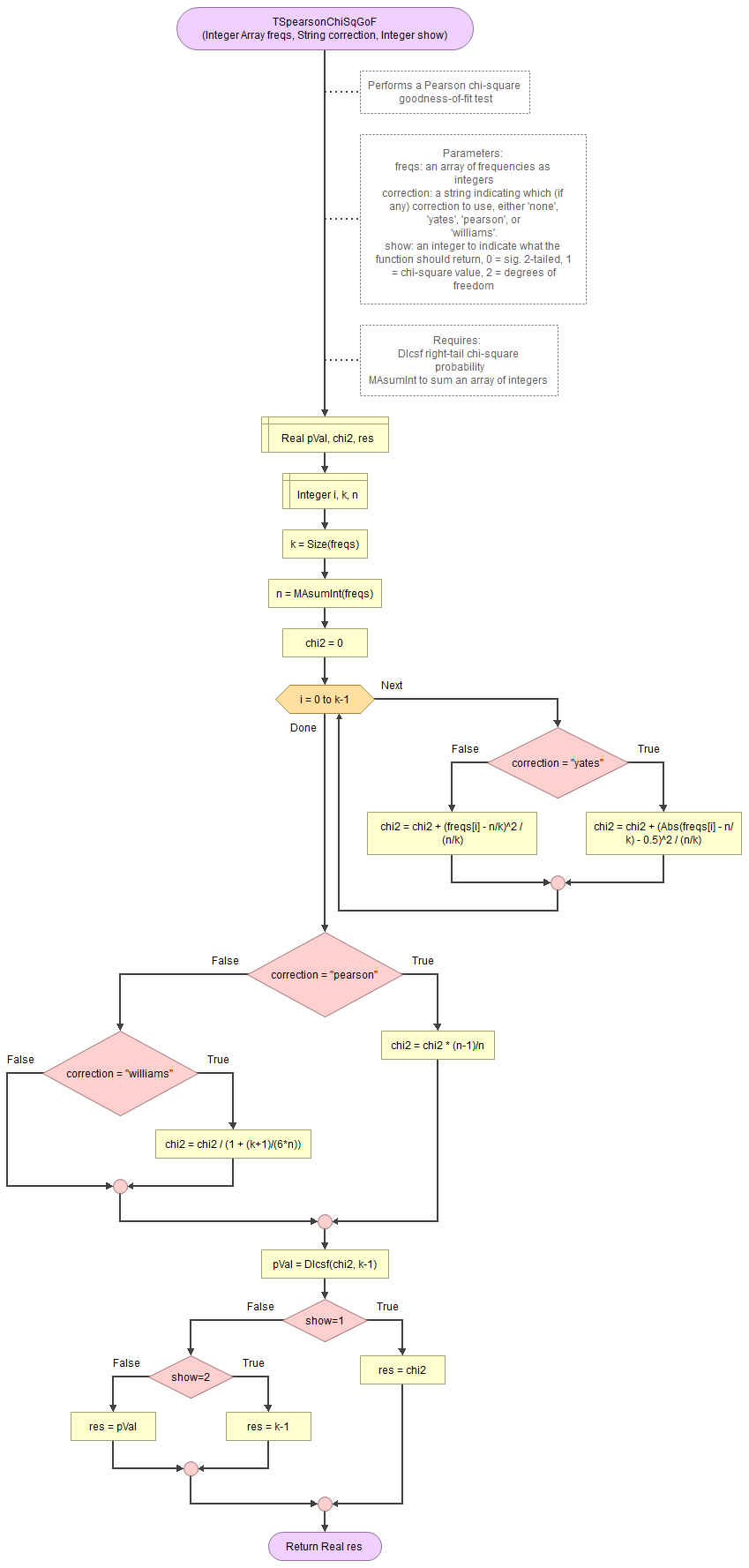
It takes as input an array of integers with the observed frequencies, a string to indicate which correction to use (either 'none', 'pearson', 'williams', or 'yates') and an integer for which output to show (0 = sig., 1=chi-square value, 2 = degrees of freedom).
It uses the function for the right-tail probabilities of the chi-square distribution and a small helper function to sum an array of integers.
Flowgorithm file: FL-TSpearsonChiSqGoF.fprg.
with Python
Jupyter Notebook from videos: TS - Pearson chi-square GoF (R).ipynb.
with stikpetP
without stikpetP
with R
Jupyter Notebook from videos: TS - Pearson chi-square GoF (S).spwb.
with stikpetR
without stikpetR
with SPSS
via One-sample
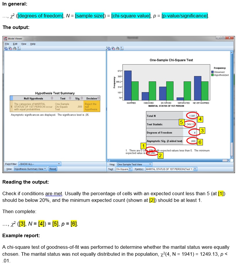
Click or hover over the thumbnail below to see where to look in the output.
Data file used in video: GSS2012-Adjusted.sav.
via Legacy dialogs
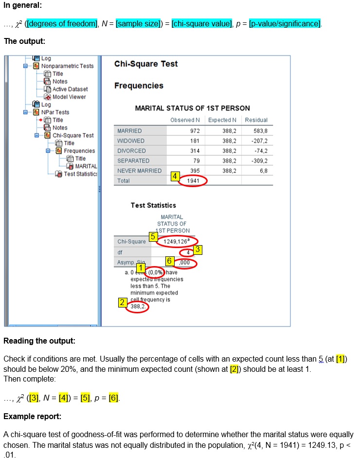
Click or hover over the thumbnail below to see where to look in the output.
Data file used in video: GSS2012-Adjusted.sav.
Manually (Formula and example)
The formula's
The Pearson chi-square goodness-of-fit test statistic (χ2):
\( \chi^{2}=\sum_{i=1}^{k}\frac{\left(O_{i}-E_{i}\right)^{2}}{E_{i}}\)
In this formula Oi is the observed count in category i, Ei is the expected count in category i, and k is the number of categories.
If the expected frequencies, are expected to be equal, then:
\(E_{i}=\frac{\sum_{j=1}^{k}O_{i}}{k}\)
The degrees of freedom is given by:
\(df=k-1\)
The probability of such a chi-square value or more extreme, can then be found using the chi-square distribution.
Example
We have the following observed frequencies of five categories:
\(O=\left(972,181,314,79,395\right)\)
Note that since there are five categories, we have k = 5. If the expected frequency for each category is expected to be equal we can use the formula to determine:
\(E_{i}=\frac{\sum_{j=1}^{k}O_{i}}{k}=\frac{\sum_{j=1}^{5}O_{i}}{5} =\frac{972+181+314+79+395}{5}\)
\(=\frac{1941}{5}=388\frac{1}{5}=388.2\)
Then we can determine the Pearson chi-square value:
\(\chi^{2}=\sum_{i=1}^{k}\frac{\left(O_{i}-E_{i}\right)^{2}}{E_{i}}=\sum_{i=1}^{5}\frac{\left(O_{i}-\frac{1941}{5}\right)^{2}}{\frac{1941}{5}}\)
\(=\frac{\left(972-\frac{1941}{5}\right)^{2}}{\frac{1941}{5}}+\frac{\left(181-\frac{1941}{5}\right)^{2}}{\frac{1941}{5}}+\frac{\left(314-\frac{1941}{5}\right)^{2}}{\frac{1941}{5}}+\frac{\left(79-\frac{1941}{5}\right)^{2}}{\frac{1941}{5}}+\frac{\left(395-\frac{1941}{5}\right)^{2}}{\frac{1941}{5}}\)
\(=\frac{\left(\frac{972\times5}{5}-\frac{1941}{5}\right)^{2}}{\frac{1941}{5}}+\frac{\left(\frac{181\times5}{5}-\frac{1941}{5}\right)^{2}}{\frac{1941}{5}}+\frac{\left(\frac{314\times5}{5}-\frac{1941}{5}\right)^{2}}{\frac{1941}{5}}+\frac{\left(\frac{79\times5}{5}-\frac{1941}{5}\right)^{2}}{\frac{1941}{5}}+\frac{\left(\frac{395\times5}{5}-\frac{1941}{5}\right)^{2}}{\frac{1941}{5}}\)
\(=\frac{\left(\frac{972\times5-1941}{5}\right)^{2}}{\frac{1941}{5}}+\frac{\left(\frac{181\times5-1941}{5}\right)^{2}}{\frac{1941}{5}}+\frac{\left(\frac{314\times5-1941}{5}\right)^{2}}{\frac{1941}{5}}+\frac{\left(\frac{79\times5-1941}{5}\right)^{2}}{\frac{1941}{5}}+\frac{\left(\frac{395\times5-1941}{5}\right)^{2}}{\frac{1941}{5}}\)
\(=\frac{\left(\frac{4860-1941}{5}\right)^{2}}{\frac{1941}{5}}+\frac{\left(\frac{905-1941}{5}\right)^{2}}{\frac{1941}{5}}+\frac{\left(\frac{1570-1941}{5}\right)^{2}}{\frac{1941}{5}}+\frac{\left(\frac{395-1941}{5}\right)^{2}}{\frac{1941}{5}}+\frac{\left(\frac{1975-1941}{5}\right)^{2}}{\frac{1941}{5}}\)
\(=\frac{\left(\frac{2919}{5}\right)^{2}}{\frac{1941}{5}}+\frac{\left(\frac{-1036}{5}\right)^{2}}{\frac{1941}{5}}+\frac{\left(\frac{-371}{5}\right)^{2}}{\frac{1941}{5}}+\frac{\left(\frac{-1546}{5}\right)^{2}}{\frac{1941}{5}}+\frac{\left(\frac{34}{5}\right)^{2}}{\frac{1941}{5}}\)
\(=\frac{\frac{\left(2919\right)^{2}}{5^{2}}}{\frac{1941}{5}}+\frac{\frac{\left(-1036\right)^{2}}{5^{2}}}{\frac{1941}{5}}+\frac{\frac{\left(-371\right)^{2}}{5^{2}}}{\frac{1941}{5}}+\frac{\frac{\left(-1546\right)^{2}}{5^{2}}}{\frac{1941}{5}}+\frac{\frac{\left(34\right)^{2}}{5^{2}}}{\frac{1941}{5}}\)
\(=\frac{\frac{8520561}{5^{2}}}{\frac{1941}{5}}+\frac{\frac{1073296}{5^{2}}}{\frac{1941}{5}}+\frac{\frac{137641}{5^{2}}}{\frac{1941}{5}}+\frac{\frac{2390116}{5^{2}}}{\frac{1941}{5}}+\frac{\frac{1156}{5^{2}}}{\frac{1941}{5}}\)
\(=\frac{8520561\times5}{1941\times5^{2}}+\frac{1073296\times5}{1941\times5^{2}}+\frac{137641\times5}{1941\times5^{2}}+\frac{2390116\times5}{1941\times5^{2}}+\frac{1156\times5}{1941\times5^{2}}\)
\(=\frac{8520561}{1941\times5}+\frac{1073296}{1941\times5}+\frac{137641}{1941\times5^{2}}+\frac{2390116}{1941\times5}+\frac{1156}{1941\times5}\)
\(=\frac{8520561+1073296+137641+2390116+1156}{1941\times5}\)
\(=\frac{12122770}{1941\times5}=\frac{2424554\times5}{1941\times5}=\frac{2424554}{1941}\approx1249.13\)
The degrees of freedom is:
\(df=k-1=5-1=4\)
To determine the signficance you then need to determine the area under the chi-square distribution curve, in formula notation:
\(\int_{x=0}^{\chi^{2}}\frac{x^{\frac{df}{2}-1}\times e^{-\frac{x}{2}}}{2^{\frac{df}{2}}\times\Gamma\left(\frac{df}{2}\right)}\)
This is usually done with the aid of either a distribution table, or some software. See the chi-square distribution section for more details.
Click here to see how to perform a Pearson chi-square test of independence...
with Python
Jupyter Notebook: TS - Pearson Chi square - Independence.ipynb
Data file used: GSS2012a.csv
with R (Studio)
Click on the thumbnail below to see where you can find each of the values mentioned in the output of the software.
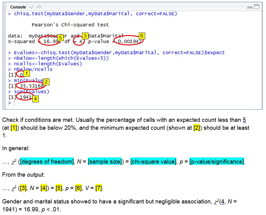
R Script: TS - Pearson Chi square - Independence.R
Data file used: GSS2012a.csv
with SPSS
Click on the thumbnail below to see where you can find each of the values mentioned in the output of the software.
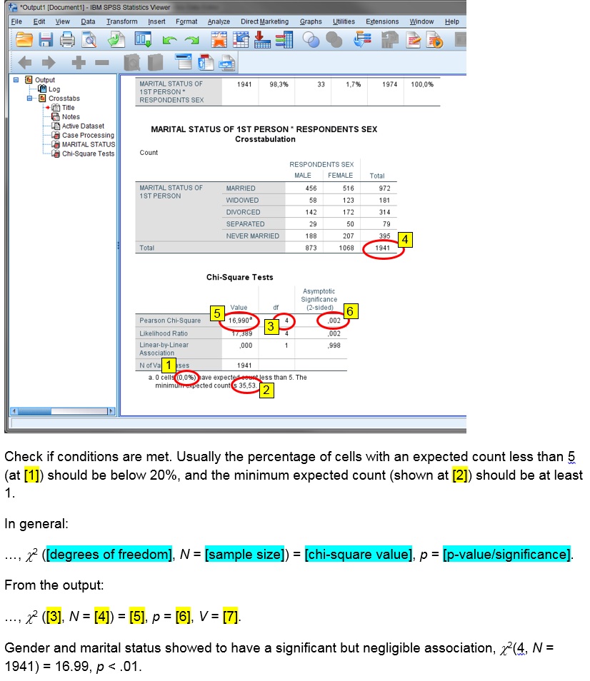
Data file used: GSS2012-Adjusted.sav
with a TI-83
Manually (Formulas and example)
Formulas
The formula for the Pearson chi-square value is:
\(\chi^2=\sum_{i=1}^{r}\sum_{j=1}^{c}\frac{(O_{i,j}-E_{i,j})^2}{E_{i,j}}\)
In this formula r is the number of rows, and c the number of columns. Oi,j is the observed frequency of row i and column j. Eij is the expected frequency of row i and column j. The expected frequency can be determined using:
\(E_{i,j}=\frac{R_i\times{C_j}}{N}\)
In this formula Ri is the total of all observed frequencies in row i, Cj the total of all observed frequencies in column j, and N the grand total of all observed frequencies. In formula notation:
\(R_i=\sum_{j=1}^{c}O_{i,j}\)
\(C_j=\sum_{i=1}^{r}O_{i,j}\)
\(N=\sum_{i=1}^{r}R_i=\sum_{j=1}^{c}C_j=\sum_{i=1}^{r}\sum_{j=1}^{c}O_{i,j}\)
The degrees of freedom is the number of rows minus one, multiplied by the number of columns minus one. In formula notation:
\(df=(r-1)\times(c-1)\)
Example
Note: different example than in rest of this page.
We are given the following table with observed frequencies.
| Brand | Red | Blue |
|---|---|---|
Nike |
10 |
8 |
Adidas |
6 |
4 |
Puma |
14 |
8 |
There are three rows, so r = 3, and two columns, so c = 2. Then we can determine the row totals:
\(R_1=\sum_{j=1}^{2}O_{1,j}=O_{1,1}+O_{1,2}=10+8=18\)
\(R_2=\sum_{j=1}^{2}O_{2,j}=O_{2,1}+O_{2,2}=6+4=10\)
\(R_3=\sum_{j=1}^{2}O_{3,j}=O_{3,1}+O_{3,2}=14+8=22\)
The column totals:
\(C_1=\sum_{i=1}^{3}O_{i,1}=O_{1,1}+O_{2,1}+O_{3,1}=10+6+14=30\)
\(C_2=\sum_{i=1}^{3}O_{i,2}=O_{1,2}+O_{2,2}+O_{3,2}=8+4+8=20\)
The grand total, all three formulas will give the same result:
\(N=\sum_{i=1}^{3}R_i=R_1+R_2+R_3=18+10+22=50\)
\(N=\sum_{j=1}^{2}C_j=C_1+C_2=30+20=50\)
\(N=\sum_{i=1}^{3}\sum_{j=1}^{2}O_{i,j}=O_{1,1}+O_{1,2}+O_{2,1}+O_{2,2}+O_{3,1}+O_{3,2}\)
\(=10+8+6+4+14+8=50\)
We can add the totals to our table:
| Brand | Red | Blue | Total |
|---|---|---|---|
Nike |
10 |
8 |
18 |
Adidas |
6 |
4 |
10 |
Puma |
14 |
8 |
22 |
| Total | 30 |
20 |
50 |
Next we calculate the expected frequencies for each cell:
\(E_{1,1}=\frac{R_1\times{C_1}}{50} =\frac{18\times{30}}{50} =\frac{540}{50} =\frac{54}{5}=10.8\)
\(E_{1,2}=\frac{R_1\times{C_2}}{50} =\frac{18\times{20}}{50} =\frac{360}{50} =\frac{36}{5}=7.2\)
\(E_{2,1}=\frac{R_2\times{C_1}}{50} =\frac{10\times{30}}{50} =\frac{300}{50} =6\)
\(E_{2,2}=\frac{R_2\times{C_2}}{50} =\frac{10\times{20}}{50} =\frac{200}{50} =4\)
\(E_{3,1}=\frac{R_3\times{C_1}}{50} =\frac{22\times{30}}{50} =\frac{660}{50} =\frac{66}{5} =13.2\)
\(E_{3,2}=\frac{R_3\times{C_2}}{50} =\frac{22\times{20}}{50} =\frac{440}{50} =\frac{44}{5} =8.8\)
An overview of these in a table might be helpful:
| Brand | Red | Blue | Total |
|---|---|---|---|
Nike |
10.8 |
7.2 |
18 |
Adidas |
6 |
4 |
10 |
Puma |
13.2 |
8.8 |
22 |
| Total | 30 |
20 |
50 |
Note that the totals remain the same. Now for the chi-square value. For each cell we need to determine:
\(\frac{(O_{i,j}-E_{i,j})^2}{E_{i,j}}\)
So again six times:
\(\frac{(O_{1,1}-E_{1,1})^2}{E_{1,1}} =\frac{(10-\frac{54}{5})^2}{\frac{54}{5}} =\frac{(\frac{50}{5}-\frac{54}{5})^2}{\frac{54}{5}} =\frac{(\frac{50-54}{5})^2}{\frac{54}{5}} =\frac{(\frac{-4}{5})^2}{\frac{54}{5}} =\frac{\frac{(-4)^2}{5^2}}{\frac{54}{5}} =\frac{\frac{16}{25}}{\frac{54}{5}} =\frac{16\times5}{25\times54} =\frac{8}{5\times27} =\frac{8}{135} \approx0.059\)
\(\frac{(O_{1,2}-E_{1,2})^2}{E_{1,2}} =\frac{(8-\frac{36}{5})^2}{\frac{36}{5}} =\frac{(\frac{40}{5}-\frac{36}{5})^2}{\frac{36}{5}} =\frac{(\frac{40-36}{5})^2}{\frac{36}{5}} =\frac{(\frac{4}{5})^2}{\frac{36}{5}} =\frac{\frac{(4)^2}{5^2}}{\frac{36}{5}} =\frac{\frac{16}{25}}{\frac{36}{5}} =\frac{16\times5}{25\times36} =\frac{4}{5\times9} =\frac{4}{45} \approx0.089\)
\(\frac{(O_{2,1}-E_{2,1})^2}{E_{2,1}} =\frac{(6-6)^2}{6} =\frac{(0)^2}{6} =\frac{0}{6} =0\)
\(\frac{(O_{2,2}-E_{2,2})^2}{E_{2,2}} =\frac{(4-4)^2}{4} =\frac{(0)^2}{4} =\frac{0}{4} =0\)
\(\frac{(O_{3,1}-E_{3,1})^2}{E_{3,1}} =\frac{(14-\frac{66}{5})^2}{\frac{66}{5}} =\frac{(\frac{70}{5}-\frac{66}{5})^2}{\frac{66}{5}} =\frac{(\frac{70-66}{5})^2}{\frac{66}{5}} =\frac{(\frac{-4}{5})^2}{\frac{66}{5}} \frac{\frac{(-4)^2}{5^2}}{\frac{66}{5}} \frac{\frac{16}{25}}{\frac{66}{5}} =\frac{16\times5}{25\times66} =\frac{8}{5\times33} =\frac{8}{165} \approx0.048\)
\(\frac{(O_{3,2}-E_{3,2})^2}{E_{3,2}} =\frac{(8-\frac{44}{5})^2}{\frac{44}{5}} =\frac{(\frac{40}{5}-\frac{44}{5})^2}{\frac{44}{5}} =\frac{(\frac{40-44}{5})^2}{\frac{44}{5}} =\frac{(\frac{-4}{5})^2}{\frac{44}{5}} \frac{\frac{(-4)^2}{5^2}}{\frac{44}{5}} \frac{\frac{16}{25}}{\frac{44}{5}} =\frac{16\times5}{25\times44} =\frac{4}{5\times11} =\frac{4}{55} \approx0.073\)
Then the chi-square value is the sum of all of these:
\(\chi^2=\sum_{i=1}^{3}\sum_{j=1}^{2}\frac{(O_{i,j}-E_{i,j})^2}{E_{i,j}} =\frac{8}{135}+\frac{4}{45}+0+0+\frac{8}{165}+\frac{4}{55}\)
\(=\frac{8\times11}{135\times11}+\frac{4\times33}{45\times33}+\frac{8\times9}{165\times9}+\frac{4\times27}{55\times27} =\frac{88}{1485}+\frac{132}{1485}+\frac{72}{1485}+\frac{108}{1485}\)
\(=\frac{88+132+72+108}{1485} =\frac{400}{1485} =\frac{80}{297} \approx0.269\)
The degrees of freedom is:
\(df=(3-1)\times(2-1)=(2)\times(1)=2\)
To determine the signficance you then need to determine the area under the chi-square distribution curve, in formula notation:
\(\int_{x=0}^{\chi^{2}}\frac{x^{\frac{df}{2}-1}\times e^{-\frac{x}{2}}}{2^{\frac{df}{2}}\times\Gamma\left ( \frac{df}{2} \right )}\)
This is usually done with the aid of either a distribution table, or some software.
Interpreting the Result
Is it appropriate to use?
First you should check if it was appropriate to use the test, since this test is unreliable if the sample sizes are small.
The criteria is often that the minimum expected count should be at least 1 and no more than 20% of cells can have an expected count less than 5. This is often referred to as 'Cochran conditions', after Cochran (1954, p. 420). Note that for example Fisher (1925, p. 83) is more strict, and finds that all cells should have an expected count of at least 5. If you don't meet the conditions you can do a
If you do not meet the criteria, there are three options. First off, are you sure you have a nominal variable, and not an ordinal one? If you have an ordinal variable, you probably want a different test. If you are sure you have a nominal variable you might be able to combine two or more categories into one larger category. If for example you asked people about their country of birth, but a few countries were only selected by one or two people, you might want to combine these simply into a category ‘other’. Be very clear though in your report that you’ve done so. Alternative you can use an exact test. For the goodness-of-fit this is a exact multinomial test of goodness-of-fit. For the test of independence a Fisher exact test (for larger than 2x2 tables this is also then known as the Fisher-Freeman-Halton Exact Test).
Reading the p-value
The assumption about the population (null hypothesis) are those expected counts, i.e. if you would research the entire population the counts would match the expected counts.
With the goodness-of-fit variation, the expected counts are often simply set so that each category is chosen evenly. For example, if the sample size was 200 and there were four categories, the expected count for each category is usually simply 200/4 = 50.
With the test of independence, the expected counts are calculated from the row and column totals. These are then the counts expected if the two variables would be independent. The null-hypothesis is then often stated as that the two variables are independent (i.e. have no influence on each other.
The test provides a p-value, which is the probability of a test statistic as from the sample, or even more extreme, if the assumption about the population would be true. If this p-value (significance) is below a pre-defined threshold (the significance level \(\alpha\) ), the assumption about the population is rejected. We then speak of a (statistically) significant result. The threshold is usually set at 0.05. Anything below is then considered low.
If the assumption is rejected, with a goodness-of-fit test, we then conclude that the categories will not be equally distributed in the population, while for a test of independence that the two variables are not independent (i.e. they have an influence on each other).
Note that if we do not reject the assumption, it does not mean we accept it, we simply state that there is insufficient evidence to reject it.
Writing the results
Both variations use the chi-square distribution. A template for tests that use this distribution would be:
χ2([degrees of freedom], N = [sample size]) = [test value], p = [p-value]
Prior to this, mention the test that was done, and the interpretation of the results. For example:
A Pearson chi-square test of goodness-of-fit showed that the marital status was not equally distributed in the population, χ2(4, N = 1941) = 1249.13, p < .001.
Round the p-value to three decimal places, or if it is below .001 (as in the example) use p < .001
You can get that chi symbol (χ) in Word by typing in the letter 'c', then select it and change the font to 'Symbol'. The square can be done by typing a '2' and make it a superscript.
APA (2019, p. 88) states to also report an effect size measure.
Prior to the test result a visualisation might be appreciated, and after the effect-size measure. We could then, if the result is significant, follow up with a post-hoc analysis. This could be for a goodness-of-fit test to determine which categories are significantly different from each other, or for a test of independence to better describe what the influence then is.
Corrections
The chi-square distribution is a so-called continuous distribution, but the observed counts are discrete. It is therefor possible to add a so-called continuity correction. I've seen three versions for this:
- Yates (1934, p. 222) (only if there are two categories (in each variable))
- Williams (1976, p. 36)
- E.S. Pearson (1947, p. 36)
Click here to see the formulas of these continuity corrections
The Yates continuity correction (cc="yates") is calculated using (Yates, 1934, p. 222):
\(\chi_{PY}^2 = \sum_{i=1}^k \frac{\left(\left|F_i - E_i\right| - 0.5\right)^2}{E_i}\)
Or adjust the observed counts with:
\(F_i^\ast = \begin{cases} F_i - 0.5 & \text{ if } F_i ≥ E_i \\ F_i + 0.5 & \text{ if } F_i < E_i \end{cases}\)
Then use these adjusted counts in the calculation of the chi-square value.
Sometimes the Yates continuity correction is written as (Allen, 1990, p. 523):
\(\chi_{PY}^2 = \sum_{i=1}^k \frac{\max\left(0, \left(\left|F_i - E_i\right| - 0.5\right)\right)^2}{E_i}\)
Which is then the same as adjusting the observed counts using:
\(F_i^\ast = \begin{cases} F_i - 0.5 & \text{ if } F_i - 0.5 > E_i \\ F_i + 0.5 & \text{ if } F_i + 0.5 < E_i \\ F_i & \text{ else } \end{cases}\)
The Pearson correction (cc="pearson") is calculated using (E.S. Pearson, 1947, p. 36):
\(\chi_{PP}^2 = \chi_{P}^{2}\times\frac{n - 1}{n}\)
The Williams correction (cc="williams") is calculated for a Goodness-of-Fit test using (Williams, 1976, p. 36):
\(\chi_{PW}^2 = \frac{\chi_{P}^2}{q}\)
With:
\(q = 1 + \frac{k^2 - 1}{6\times n\times df}\)
While for a test of independence the formula of q changes to (Williams, 1976, p. 36; McDonald, 2014):
\(q = 1+\frac{\left(n\times \left(\sum_{i=1}^r \frac{1}{R_i}\right) - 1\right)\times \left(n\times\left(\sum_{j=1}^c \frac{1}{C_i}\right) - 1\right)}{6\times n \times\left(r - 1\right)\times\left(c - 1\right)}\)
Note that the Yates correction has been shown to be too conservative and is often discouraged to be used (see Haviland (1990) for a good starting point on this).
Next step and Alternatives
APA (2019, p. 88) states to also report an effect size measure with statistical tests. With a Goodness-of-Fit test this could be:
If the test is significant a post-hoc analysis to pin-point which category is significantly different could be used. The post-hoc anlysis for a goodness-of-fit test is discussed here.
There are quite a few tests that can be used with a single or two nominal variables:
- Exact Test (Multinomial for GoF, Fisher for 2x2 and Fisher-Hamiton for larger tables)
- Pearson Chi-Square
- Neyman
- (Modified) Freeman-Tukey
- Cressie-Read / Power Divergence
- Freeman-Tukey-Read
- G / Likelihood Ratio / Wilks
- Mod-Log Likelihood
The Pearson chi-square is probably the most famous and used one. Neyman swops the observed and expected counts in Pearson's formula. Freeman-Tukey attempts to smooth the chi-square distribution by using a square root transformation, while the G test uses a logarithm transformation. Cressie-Read noticed that all the others ones can be placed in a generic format and created a whole family of tests. For the goodness-of-fit tests Read also proposed an alternative generalisation.
As for goodness-of-fit tests, McDonald (2014, p. 82) suggests to always use the exact test as long as the sample size is less than 1000 (which was just picked as a nice round number, when n is very large the exact test becomes computational heavy even for computers). Lawal (1984) continued some work from Larntz (1978) and compared the modified Freeman-Tukey, G-test and the Pearson chi-square test, and concluded that for small samples the Pearson test is preferred, while for large samples either the Pearson or G-test. Making the Freeman-Tukey test perhaps somewhat redundant.
Tests
![]()

Google adds