Hedges g

Introduction

Hedges g is a correction of Cohen d. Similar as Cohen d, it therefor compares the difference between two means. It informs on how many standard deviations the difference is. There are three variations of this effect size measure:

one-sample, to compare the sample mean with an hypothesized mean
independent-samples, to compare two sample means, each from a different group (e.g. national vs. international)
paired samples, to compare two sample means from paired data (e.g. pre-test and post-test)

There is an 'exact' correction from Hedges, and an approximate version. Durlak and also Xue give other corrections for Cohen's d, so these could be considered alternative versions of Hedges g.

Obtaining the Measure

Click here to see how to obtain Hedges g for a one-sample test.

with Excel

Excel file: ES - Hedges g (one-sample).xlsm.

with stikpetE

without stikpetE add-in

with Flowgorithm

A flowgorithm for Hedges g (one-sample) in Figure 1.

Flowgorithm Hedges g (one-sample)

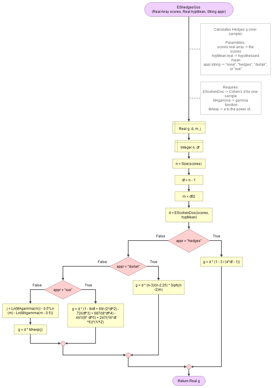
It takes as input paramaters the scores, the hypothesized mean, and which approximation to use (if any).

It uses a function for Cohen's d (EScohenDos), the gamma function (MAgamma), and the e power function (MAexp). Cohen's d function requires in turn the mean (CEmean) and standard deviation (VAsd) functions, which make use of the MAsumReal (sum of real values) function. The gamma function needs the factorial function (MAfact)

Flowgorithm file: FL-EShedgesGos.fprg.

with Python

Jupyter Notebook used in video: ES - Hedges g (one-sample) (P).ipynb.

with stikpetP

without stikpetP library

with R (Studio)

Jupyter Notebook used in video: ES - Hedges g (one-sample) (R).ipynb.

with stikpetR

without stikpetR

with SPSS

This has become available in SPSS 27. There is no option in earlier versions of SPSS to determine Hedges g, but it can easily be calculated using the 'Compute variable' option as shown in the video.

SPSS 27 or later

Datafile used in video: GSS2012-Adjusted.sav

SPSS 26 or earlier

Datafile used in video: GSS2012-Adjusted.sav

manually (Formula)

The exact formula for Hedges g is (Hedges, 1981, p. 111):

\(g = d\times\frac{\Gamma\left(m\right)}{\Gamma\left(m-0.5\right)\times\sqrt{m}}\)

With \(d\) as Cohen's d, and \(m = \frac{df}{2}\), where \(df=n-1\)

The \(\Gamma\) indicates the gamma function, defined as:

\(\Gamma\left(a=\frac{x}{2}\right)=\begin{cases} \left(a - 1\right)! & \text{ if } x \text{ is even}\ \frac{\left(2\times a\right)!}{4^a\times a!}\times\sqrt{\pi} & \text{ if } x \text{ is odd}\end{cases}\)

Because the gamma function is computational heavy there are a few different approximations.

Hedges himself proposed (Hedges, 1981, p. 114):

\(g^* \approx d\times\left(1 - \frac{3}{4\times df-1}\right)\)

Durlak (2009, p. 927) shows another factor to adjust Cohens d with:

\(g^* = d\times\frac{n-3}{n-2.25}\times\sqrt{\frac{n-2}{n}}\)

Xue (2020, p. 3) gave an improved approximation using:

\(g^* = d\times\sqrt[12]{1-\frac{9}{df}+\frac{69}{2\times df^2}-\frac{72}{df^3}+\frac{687}{8\times df^4}-\frac{441}{8\times df^5}+\frac{247}{16\times df^6}}\)

Note 1. You might come across the following approximation: (Hedges & Olkin, 1985, p. 81)

\(g^* = d\times\left(1-\frac{3}{4\times n - 9}\right)\)

This is an alternative but equal method, but for the paired version. In the paired version we set df = n - 2, and if we substitute this in the Hedges version it gives the same result. The denominator of the fraction will then be:

\(4\times df - 1 = 4 \times\left(n-2\right) - 1 = 4\times n-4\times2 - 1 = 4\times n - 8 - 1 = 4\times n - 9\)

Note 2. Often for the exact formula 'm' is used for the degrees of freedom, and the formula will look like:

\(g = d\times\frac{\Gamma\left(\frac{m}{2}\right)}{\Gamma\left(\frac{m-1}{2}\right)\times\sqrt{\frac{m}{2}}}\)

Note 3: Alternatively the natural logarithm gamma can be used by using:

\(j = \ln\Gamma\left(m\right) - 0.5\times\ln\left(m\right) - \ln\Gamma\left(m-0.5\right)\)

and then calculate:

\(g = d\times e^{j}\)

In the formula for \(j\) we still use \(m = \frac{df}{2}\).

Click here to see how to obtain Hedges g for independent samples.

with Excel

Excel file: ES - Cohen d and Hedges g (ind samples) (E).xlsm

with stikpetE

To Be Made

without stikpetE

To Be Made

with Python

Jupyter Notebook: ES - Cohen d and Hedges g (ind samples) (P).ipynb

with stikpetP

To Be Made

without stikpetP

To Be Made

with R

Jupyter Notebook: ES - Cohen d and Hedges g (ind samples) (R).ipynb

with stikpetR

To Be Made

without stikpetR

To Be Made

manually (Formula)

The formula for the uncorrected Hedges g (Hedges, 1981, p. 110) is the same as that for Cohen d_s (Cohen, 1988, p. 66):

\(g = \frac{\bar{x}_1 - \bar{x}_2}{s_p}\)

With:

\(s_p = \sqrt{\frac{SS_1^2 + SS_2^2}{n - 2}}\)

\(SS_i = \sum_{j=1}^{n_i} \left(x_{i,j} - \bar{x}_i\right)^2\)

\(\bar{x}_i = \frac{\sum_{j=1}^{n_i} x_{i,j}}{n_i}\)

This uses the formula as shown above for \(s_p\). However, sometimes the unweighted version is used:

\(s_p = \sqrt{\frac{s_1^2 + s_2^2}{2}}\)

Hedges proposes the following exact bias correction (Hedges, 1981, p. 111):

\(g_{c} = g \times\frac{\Gamma\left(m\right)}{\Gamma\left(m - \frac{1}{2}\right)\times\sqrt{m}}\)

With:

\(m = \frac{df}{2}\)

\(df = n_1 + n_2 - 2= n - 2\)

The formula used for the approximation for this correction from Hedges (1981, p. 114):

\(g_c = g \times\left(1 - \frac{3}{4\times df - 1}\right)\)

This approximation can also be found in Hedges and Olkin (1985, p. 81) and Cohen (1988, p. 66)

The formula used for the approximation from Durlak (2009, p. 927):

\(g_c = g \times\frac{n - 3}{n - 2.25} \times\sqrt{\frac{n - 2}{n}}\)

The formula used for the approximation from Xue (2020, p. 3):

\(g_c = g \times \sqrt[12]{1 - \frac{9}{df} + \frac{69}{2\times df^2} - \frac{72}{df^3} + \frac{687}{8\times df^4} - \frac{441}{8\times df^5} + \frac{247}{16\times df^6}}\)

Symbols used:

\(x_{i,j}\) the j-th score in category i
\(n_i\) the number of scores in category i
\(df\) the degrees of freedom
\(n\) the sample size (i.e. the number of scores)
\(\Gamma\left(\dots\right)\) the gamma function

Interpretation

Hedges g can range from negative infinity to positive infinity. A zero would indicate no difference at all between the two means, the higher the value the larger the effect.

Various authors have proposed rules-of-thumb for the classification of Cohen d, and since Hedges g is a correction for Cohen d, we could use the same classifications. A few are listed in table 1.

Table 1
Rule of thumb for Cohen’s d
\|d\|	Brydges (2019, p. 5)	Cohen (1988, p. 40)	Sawilowsky (2009, p. 599)	Rosenthal (1996, p. 45)	Lovakov and Agadullina (2021, p. 501)
0.00 < 0.10	negligible	negligible	negligible	negligible	negligible
0.10 < 0.15	negligible		very small		negligible
0.15 < 0.20	small		very small		small
0.20 < 0.35		small	small	small	small
0.35 < 0.40					medium
0.40 < 0.50	medium
0.50 < 0.65		medium	medium	medium
0.65 < 0.75					large
0.75 < 0.80	large
0.80 < 1.20		large	large	large
1.20 < 1.30			very large	large
1.30 < 2.00			very large	very large
2.00 or more			huge	very large

Note that these are just some rule-of-thumb and can differ depending on the field of the research.

Links to parts

Google adds