
Cramér V
Introduction
Cramér's V (Cramér, 1946, p. 282) is an extension of the Phi-Coefficient, which is only for 2x2 tables. It takes the chi-square value, and divides it by the maximum possible chi-square value, and takes the square root out of this. This ensures it will always be between 0 and 1.
It gives an estimate of how well the data then fits the expected values, where 0 would indicate that they are exactly equal. If you use the equal distributed expected values the maximum value would be 1, otherwise it could actually also exceed 1.
The effect size was originally intended for tests of independence, but can also be used for goodness-of-fit tests (Kelley & Preacher, 2012, p. 145; Mangiafico, 2016, p. 474).
Obtaining the Measure
Click here to see how to obtain Cramér's V for goodness-of-fit test.
with Excel
Excel file: ES - Cramer's V (GoF) (E).xlsm
with stikpetE add-in:
without stikpetE add-in:
with Flowgorithm
A basic implementation for Cramér's V in the flowchart in figure 1
Figure 1
Flowgorithm for Cramér's V
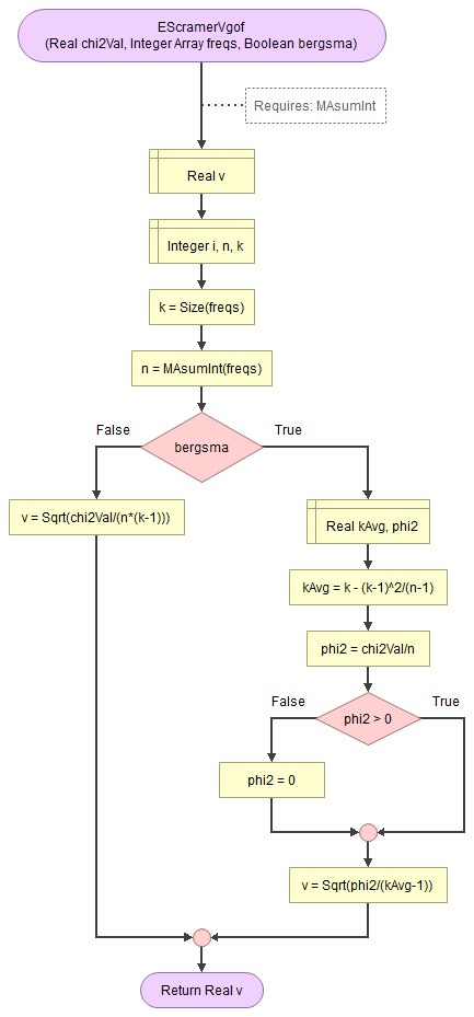
It takes as input the chi-square value, an array of integers with the observed frequencies, and a boolean to indicate to use the Bergsma correction.
It uses a small helper function to sum an array of integers.
Flowgorithm file: FL-EScramerVgof.fprg.
with Python
Jupyter Notebook: ES - Cramers V (GoF) (P).ipynb
with stikpetP library:
without stikpetP library:
with R (Studio)
Jupyter Notebook: ES - Cramers V (GoF) (R).ipynb
with stikpetR library:
without stikpetR library:
with SPSS
Unfortunately SPSS does not have a method to determine Cramér's V directly from the GUI, however the calculation is not very difficult once you have the output from the previous part.
The video below shows how this could be done with a bit of help from Excel
Online calculator
Enter the requested information below:
Manually (formula and example)
Formula
The formula for Cramér's V is:
\(V=\sqrt\frac{\chi^{2}}{n\times df}\)
In the above formula \(\chi^2\) is the chi-square test value, \(n\) is the total sample size, and \(df\) is the degrees of freedom, determined by \(df=k-1\). \(k\) is the number of categories.
Example.
If we have a chi-square value of 1249.13, a total sample size of 1941, and had five categories, we can first determine the degrees of freedom (df):
\(df = k - 1 = 5 - 4 = 4\)
Then we can fill out all values in the formula for Cramér's V:
\(V=\sqrt\frac{\chi^{2}}{n\times df}=\sqrt\frac{1249.13}{1941\times4}=\sqrt\frac{1249.13}{7764}\approx\sqrt{0.1609}\approx0.4011\)
Click here to see how to obtain Cramer's V for a test of independence.
with Excel
with Python
with R (Studio)
with SPSS
Online calculator
Enter the requested information below:
Manually (formulas and example)
Formulas
The formula for Cramer's V is:
\(V=\sqrt{\frac{\chi^2}{n\times(\textup{MIN}(r,c)-1)}}\)
In this formula χ2 is the chi-square value, n the total sample size, r the number of rows (or categories in the 1st variable), and c the number of columns (or categories in the 2nd variable). MIN(r,c) simply indicates to take the minimum from r and c, so the lowest of the two.
Example
Note this is a different example than the one used in the rest of this section, but the same as the one used in the example of the manual calculation of the test.
We are given the following table with observed frequencies.
| Brand | Red | Blue |
|---|---|---|
Nike |
10 |
8 |
Adidas |
6 |
4 |
Puma |
14 |
8 |
There are three rows, so r = 3, and two columns, so c = 2. The total sample size is:
\(n=10+8+6+4+14+8=50\)
The chi-square value has also been calculated (see example in manual calculation of the test in the previous section):
\(\chi^2=\frac{80}{297} \approx0.269\)
The minimum of the rows and columns is 2 (the columns):
\(\textup{MIN}(r,c)=\textup{MIN}(3,2)=2\)
We can now fill out the formula for Cramer's V:
\(V=\sqrt{\frac{\chi^2}{n\times(\textup{MIN}(r,c)-1)}} =\sqrt{\frac{\frac{80}{297}}{50\times(2-1)}} =\sqrt{\frac{\frac{80}{297}}{50}}\)
\(=\sqrt{\frac{80}{297\times50}} =\sqrt{\frac{8}{297\times5}} =\frac{1}{297\times5}\sqrt{8\times297\times5}\)
\(=\frac{1}{1485}\sqrt{2\times4\times9\times33\times5} =\frac{1}{1485}\sqrt{4}\times\sqrt{9}\times\sqrt{2\times33\times5}\)
\(=\frac{1}{1485}\times2\times3\times\sqrt{330} =\frac{6}{1485}\sqrt{330} =\frac{2}{495}\sqrt{330} \approx0.073\)
Interpretation
Table 1 shows a rule-of-thumb interpertation for Cramer's v.
| df* | Negligible | Small | Medium | Large |
|---|---|---|---|---|
| 1 | 0 < 0.100 | 0.100 < 0.300 | 0.300 < 0.500 | ≥ 0.500 |
| 2 | 0 < 0.071 | 0.071 < 0.212 | 0.212 < 0.354 | ≥ 0.354 |
| 3 | 0 < 0.058 | 0.058 < 0.173 | 0.173 < 0.289 | ≥ 0.289 |
| 4 | 0 < 0.050 | 0.050 < 0.150 | 0.150 < 0.250 | ≥ 0.250 |
| x | 0.1 / SQRT(x) | 0.3 / SQRT(x) | 0.5 / SQRT(x) | |
| Note: Adapted from Statistical power analysis for the behavioral sciences (2nd ed., pp. 227) by J. Cohen, 1988, L. Erlbaum Associates. | ||||
The table is based on a conversion from Cohen w to Cramer's v (Cohen, 1988, p. 223). The 'df*' is either the number of rows minus one, or the number of columns minus one, whichever is smaller. In case of a goodness-of-fit it is simply the number of categories minus one.
As a finishing touch, Cramér's V can be adjusted using a bias-correction. In case you are interested the formula is a as follows (Bergsma, 2013, pp. 324-325).
\(V_B = \sqrt{\frac{\tilde{\varphi}^2}{\text{min}\left(\tilde{r}, \tilde{c}\right) - 1}}\)
With:
\(\tilde{\varphi}^2 = \text{max}\left(0,\varphi^2 - \frac{\left(r - 1\right)\times\left(c - 1\right)}{n - 1}\right)\)
\(\tilde{r} = r - \frac{\left(r - 1\right)^2}{n - 1}\)
\(\tilde{c} = r - \frac{\left(c - 1\right)^2}{n - 1}\)
\(\varphi^2 = \frac{\chi^{2}}{n}\)

Google adds