Quantiles

Explanation

The median is the value in the middle of a sorted list of scores, i.e. the value for which 50% of the scores is equal or lower, and 50% in higher or lower. We could of course also split the data into four parts, each having 25% of the data. This results in the so-called quartiles.

A bit odd, but there are five quartiles. The 0th quartile is the minimum value, the 1st the value at 25%, the 2nd at 50% (equal to the median), the 3rd at 75%, and the 4th at the maximum (100%). One could argue about the 0th quartile being the minimum, alternative we could simply not define it. The term lower quartile and higher quartile (McAlister, 1879, p. 374) or upper quartile (Galton, 1881, p. 245) are also used for the first and third quartile.

Unlike with the median, there are a lot of different methods to go about this (in the formula section I've listed 20 of them). They have slightly different results, and for large sample sizes this will usually not have a big impact. Just to show one difference figure 1 illustrates two different methods to determine what the quartiles should be.

Figure 1
Two options for quartiles for scores 1 to 9

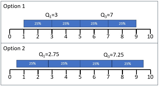
Both options have the same median, but the quartiles are different. One special mentioning is the method from Tukey who didn't use the term quartiles but hinges (Tukey, 1977, p. 33). The approach from Tukey is illustrated in figure 2.

Figure 1
Illustration of Tukey's Hinges

Quantiles (Kendall, 1940, p. 83) take the quartiles idea a step further and in essence just go for any percentage you want. If you divide by ranges of 20% you get quintiles (Fisher et al., 1922, p. 340), by 10% decentiles (Galton, 1881, p. 245), by 1% percentiles (Galton, 1885, p. 276), etc.

Obtaining the Measure

with Excel

Excel file: ME - Quartiles and Quantiles (E).xlsm

using stikpetE

without using stikpetE, using built-in functions

without using stikpetE, without built-in functions

without using stikpetE, for non-numerical data

with Python

Notebook: ME - Quartiles and Quantiles (P).ipynb

using stikpetP

without using stikpetP, using Pandas or Numpy

without using stikpetP, without 3rd party libraries

with R

Notebook from video: ME - Quartiles and Quantiles (R).ipynb

using stikpetR

without using stikpetR

without using stikpetR, all possible methods

with SPSS

Formula

For the inclusive method, the index of the first and third quartile can be found using:

\(i = \begin{cases} \frac{n+2}{4} & \text{ if } n \text{ mod } 2 = 0 \\ \frac{n+3}{4} & \text{ else } \end{cases}\)

\(i = \begin{cases} \frac{3\times n +2}{4} & \text{ if } n \text{ mod } 2 = 0 \\ \frac{3\times n+1}{4} & \text{ else } \end{cases}\)

For the exlusive method, the index of the first and third quartile can be found using:

\(i = \begin{cases} \frac{n+2}{4} & \text{ if } n \text{ mod } 2 = 0 \\ \frac{n + 1}{4} & \text{ else } \end{cases}\)

\(i = \begin{cases} \frac{3\times n +2}{4} & \text{ if } n \text{ mod } 2 = 0 \\ \frac{3\times n + 3}{4} & \text{ else } \end{cases}\)

The inclusive method could be found in Tukey (1977, p. 32), Siegel and Morgan (1996, p. 77) or Vining (1998, p. 44). Tukey referred to this as hinges, rather than quartiles. The exclusive method in Moore and McCabe (1989, p. 33) or Joarder and Firozzaman (2001, p. 88).

Others use a proportion of the data (\(p\)). These can then be used for any quantile. For a first quartile \(p = \frac{1}{4}\), and for a third quartile \(p = \frac{3}{4}\). The index of the quantile \(i\) can then be found in different ways, depending on your source.

Table 1.
*index from proportion methods*
Label	i
SAS1	\(n\times p\)
SAS4	\(\left(n + 1\right)\times p\)
HL	\(n\times p + \frac{1}{2}\)
Excel	\(\left(n - 1\right)\times p + 1\)
HF8	\(\left(n + \frac{1}{3}\right)\times p + \frac{1}{3}\)
HF9	\(\left(n + \frac{1}{4}\right)\times p + \frac{3}{8}\)

If the resulting index \(i\) is an integer there are two options:

use that integer as index, i.e. \(Q_p = x_i\)
use the midpoint between the score with that index and the next integer, i.e. \(Q_p = \frac{x_{i} + x_{i+1}}{2}\)

If the resulting index is not an integer there are a few different variations

round down \(\lfloor\dots\rfloor\)
round up \(\lceil\dots\rceil\)
use bankers rounding \(\left<\dots\right>\)
round to the nearest integer \(\left[\dots\right]\)
round half always down, rest normal \(\lfloor\dots\rceil\)
take the midpoint
use linear interpolation

The midpoint can be calculated using:

\(Q_p = \frac{x_{\lfloor i\rfloor} + x_{\lceil i \rceil}}{2} \)

The linear interpolation uses

\(Q_p = \left(i - \lfloor i\rfloor \right)\times\left(x_{\lceil i \rceil} - x_{\lfloor i \rfloor} \right) + x_{\lfloor i \rfloor}\)

If the index is not an integer the method used can even change depending on if the requested quantile is above or below the median.

Table 2.
*quantile methods overview*
method	indexing	i is int	p < 0.5	p > 0.5
sas1	sas1	use int	linear	linear
sas2	sas1	use int	bankers	bankers
sas3	sas1	use int	up	up
sas5	sas1	midpoint	up	up
hf3b	sas1	use int	nearest	halfdown
sas4	sas4	use int	linear	linear
ms	sas4	use int	nearest	halfdown
Lohninger	sas4	use int	nearest	nearest
hl2	hl	use int	linear	linear
hl1	hl	use int	midpoint	midpoint
maple2	hl	use int	down	down
excel	excel	use int	linear	linear
pd2	excel	use int	down	down
pd3	excel	use int	up	up
pd4	excel	use int	halfdown	nearest
pd5	excel	use int	midpoint	midpoint
hf8	hf8	use int	linear	linear
hf9	hf9	use int	linear	linear

For the naming was used:

sas, referring to the SAS software package
hf, short for Hyndman and Fan
hl, short for Hog and Ledolter
ms, short for Mendenhall and Sincich
jf, short for Joarder and Firozzaman
maple, referring to the Maple software
pd, referring to Python's pandas library

SAS-1 (1990, p. 626) = Parzen (1979, p. 108) = Hyndman and Fan v4 (1996, p. 363) = Maple-3 (n.d.) = interpolated inverted cdf (Numpy, n.d.):

\(Q_p = \left(i - \lfloor i\rfloor \right)\times\left(x_{\lceil i \rceil} - x_{\lfloor i \rfloor} \right) + x_{\lfloor i \rfloor}\)
with \(i = n\times p\)

Below all the formulas for the different methods, with the source and alternative namings

SAS-2 (1990, p. 626) = Hyndman and Fan v3 (1996, p. 362)

\(Q_p = x_{\lfloor i \rceil}\)
with SAS-1 indexing: \(i = n\times p\)

SAS-3 (1990, p. 626) = Hyndman and Fan v1 (1996, p. 362) = Maple-1 (n.d.) = inverted_cdf (Numpy, n.d.)

\(Q_p = x_{\lceil i \rceil}\)
with SAS-1 indexing: \(i = n\times p\)

SAS-5 (1990, p. 626) = Hyndman and Fan v2 (1996, p. 362) = averaged_inverted_cdf (Numpy, n.d.)

\(Q_p = \begin {cases} \frac{x_i + x_{i+1}}{2} & i = \lfloor i \rfloor \\ x_{\lceil i \rceil} & i \neq \lfloor i \rfloor \end{cases} \)
with SAS-1 indexing: \(i = n\times p\)

hf3b = Closest observation (Numpy, n.d.)

\(Q_p = \begin {cases} x_{\left[i\right]} & p < 0.5 \\ x_{\left< i \right>} & p > 0.5 \end{cases} \)
with SAS-1 indexing: \(i = n\times p\)
Note: The naming hf3b comes from Python’s numpy library and the function quantile. It claims to be the third method from Hyndman & Fan, but that is actually incorrect.

SAS-4 (1990, p. 626) = Hyndman and Fan v6 (1996, p. 363) = Snedecor (1940, p. 43) = Maple-5 (n.d.) = weibull (Numpy, n.d.)

\(Q_p = \left(i - \lfloor i\rfloor \right)\times\left(x_{\lceil i \rceil} - x_{\lfloor i \rfloor} \right) + x_{\lfloor i \rfloor}\)
with SAS-4 indexing: \(i = \left(n + 1\right)\times p\)
Note: Hyndman and Fan reference Weibull (1939) but couldn’t really find it in there

Mendenhall and Sincich (1992, p. 35)

\(Q_p = \begin {cases} x_{\left[i\right]} & p < 0.5 \\ x_{\left< i \right>} & p > 0.5 \end{cases} \)
with SAS-4 indexing: \(i = \left(n + 1\right)\times p\)

Lohninger (n.d.)

\(Q_p = x_{\left[ i \right]}\)
with SAS-4 indexing: \(i = \left(n + 1\right)\times p\)

Hogg and Ledolter v2 (1992, p. 21) = Hazen (1914, p. ?) = Hyndman and Fan v5 (1996, p. 363) = Maple-4 (n.d.)

\(Q_p = \left(i - \lfloor i\rfloor \right)\times\left(x_{\lceil i \rceil} - x_{\lfloor i \rfloor} \right) + x_{\lfloor i \rfloor}\)
with HL indexing: \(i = n\times p + \frac{1}{2}\)

Hogg and Ledolter v1 (1992, p. 21) = Hazen (1914, p. ?)

\(Q_p = \frac{x_{\lfloor i\rfloor} + x_{\lceil i\rceil}}{2}\)
with HL indexing: \(i = n\times p + \frac{1}{2}\)

Maple-2 (n.d.)

\(Q_p = \lfloor i\rfloor\)
with HL indexing: \(i = n\times p + \frac{1}{2}\)

Excel = Hyndman and Fan v7 (1996, p. 363) = linear (Numpy, n.d.) = Maple-6 (n.d.) = Pandas v1 (n.d.) = Gumbel (1939, p. ?)

\(Q_p = \left(i - \lfloor i\rfloor \right)\times\left(x_{\lceil i \rceil} - x_{\lfloor i \rfloor} \right) + x_{\lfloor i \rfloor}\)
with Excel indexing: \(i = \left(n - 1\right)\times p + 1\)

lower (Numpy, n.d.; Pandas, n.d.)

\(Q_p = x_{\lfloor i \rfloor}\)
with Excel indexing: \(i = \left(n - 1\right)\times p + 1\)

higher (Numpy, n.d.; Pandas, n.d.)

\(Q_p = x_{\lceil i \rceil}\)
with Excel indexing: \(i = \left(n - 1\right)\times p + 1\)

nearest (Numpy, n.d.; Pandas, n.d.)

\(Q_p = x_{\left[i\right]}\)
with Excel indexing: \(i = \left(n - 1\right)\times p + 1\)

midpoint (Numpy, n.d.; Pandas, n.d.)

\(Q_p = \frac{x_{\lfloor i\rfloor} + x_{\lceil i\rceil}}{2}\)
with Excel indexing: \(i = \left(n - 1\right)\times p + 1\)

Hyndman and Fan v8 (1996, p. 363) = Maple-7 (n.d.) = median_unbiased (Numpy, n.d.)

\(Q_p = \left(i - \lfloor i\rfloor \right)\times\left(x_{\lceil i \rceil} - x_{\lfloor i \rfloor} \right) + x_{\lfloor i \rfloor}\)
with HF8 indexing: \(i = \left(n + \frac{1}{3}\right)\times p + \frac{1}{3}\)

Hyndman and Fan v9 (1996, p. 364) = Maple-8 (n.d.) = normal_unbiased (Numpy, n.d.)

\(Q_p = \left(i - \lfloor i\rfloor \right)\times\left(x_{\lceil i \rceil} - x_{\lfloor i \rfloor} \right) + x_{\lfloor i \rfloor}\)
with HF9 indexing: \(i = \left(n + \frac{1}{4}\right)\times p + \frac{3}{8}\)

Links to parts

Google adds