
Mode
Note: click here if you prefer to watch a video about the mode than read
A measure of central tendency attempts to let one number represent the data as good as possible. The most commonly used measure of central tendency for a nominal variable is the mode. This is defined as “the abscissa corresponding to the ordinate of maximum frequency” (Pearson, 1895, p. 345). A more modern definition would be “the most common value obtained in a set of observations” (Weisstein, 2002). The word mode might even come from the French word 'mode' which means fashion. Fashion is what most people wear, so the mode is the option most people chose.
If one category has the highest frequency this category will be the modal category and if two or more categories have the same highest frequency each of them will be the mode. If there is only one mode the set is sometimes called unimodal, if there are two it is called bimodal, with three trimodal, etc. For two or more, the term multimodal can also be used.
One small controversy exists if all categories have the same frequency. In this case none of them has a higher occurence than the others, so none of them would be the mode (see for example Spiegel & Stephens, 2008, p. 64, Larson & Farber, 2014, p. 69). On a rare occasion someone might argue that if all categories have the same frequency, then all categories are part of the mode since they all have the highest frequency. A third interpretation was found on this site, where if the frequency is one for each category, then there is no mode, and if the frequency is more than one but the same, then all of them are the mode.
The mode can easily be spotted from a bar-chart (the category(s) with the highest bar), or a frequency table (the category(s) with the highest frequency). Software packages can also determine the mode, but be careful on how they deal with multiple modes.
Click here to see how to determine the mode, with Excel, Python, R, or SPSS.
with R (Studio)
Jupyter Notebook: CE - Mode (R).ipynb
with stikpetR library:
without stikpetR library:
Note that when having binned data (e.g. 0 < 10, 10 < 20, 20 < 30, etc.) the mode is not the category with the highest frequency, but the one (or ones) with the highest frequency density. Either the bin itself, the midpoint or a quadratic midpoint could then be labelled as the mode.
Click here to see how to determine the mode for binned data, with Excel, Python, R, or SPSS.
with SPSS
to be made
Formula Quadratic Mean
to be made
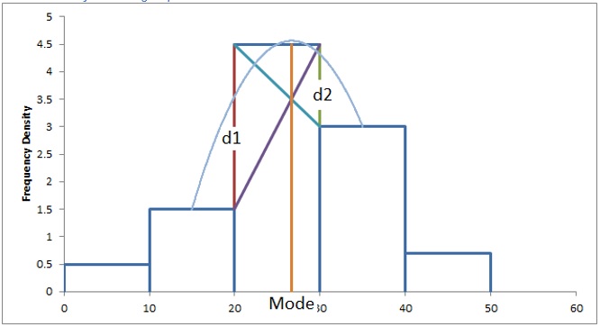
\(QM_i = LB_m + \\frac{d_1}{d_1 + d_2} \times \left(UB_m + LB_m\right)\)
With:
\(d_1 = \begin {cases} FD_m - FD_{m - 1} & m > 1 \\ FD_m & m = 1 \end {cases}\)
\(d_2 = \begin {cases} FD_m - FD_{m + 1} & m < k \\ FD_m & m = k \end {cases}\)
Symbols used:
- \(m\), the bin number of the bin with the mode.
- \(LB_i\), the lower bound of bin \(i\).
- \(UB_i\), the upper bound of bin \(i\).
- \(FD_i\), the frequency density of bin \(i\).
- \(k\), the number of bins.
The idea behind this formula is to estimate the peak in the diagram if the data would be smoothed (like a curve), by plotting the quadratic function that goes through the middle of the previous class, the modal class and the next class. Figure 1 shows how this mode can be found visually.
Figure 1
Mode using Quadratic Mean
It is a good habit to also report a measure of dispersion besides a measure of central tendancy. One possible measure of dispersion that could be reported with the mode is the variation ratio.

Google adds