
One-Sample Sign Test
Introduction
Would the majority of people in the population not see accounting as very scientific? The majority would be more than 50% of the people, so in other words, is the median (the score in the middle) in the population significantly different from 2.5 (since 2 = pretty scientific, and 3 = not scientific)?
Three tests could be used for this, the first does exactly what is described above, and is known as a sign-test, however another test is more frequently used and has a lot scarier name: one-sample Wilcoxon signed rank test (Wilcoxon, 1945). This second test uses rankings (it ranks the scores) and because of this might give a slightly different result. However the Wilcoxon signed rank test requires the data to be symmetrical, while the sign test does not. The third is a trinomial test, it is similar as a sign test but doesn't exclude the values tied with the hypothesized value.
The one-sample sign test is actually a binomial test, using:
- the number of scores unequal to the hypothesized median as number of trials,
- the minimum of the number of the scores that were above the hypothesized median, and those below, as the number of successes,
- 0.5 as the probability of success on each trial.
Performing the Test
with Flowgorithm
A flowgorithm for the one-sample sign test is shown in Figure 1.
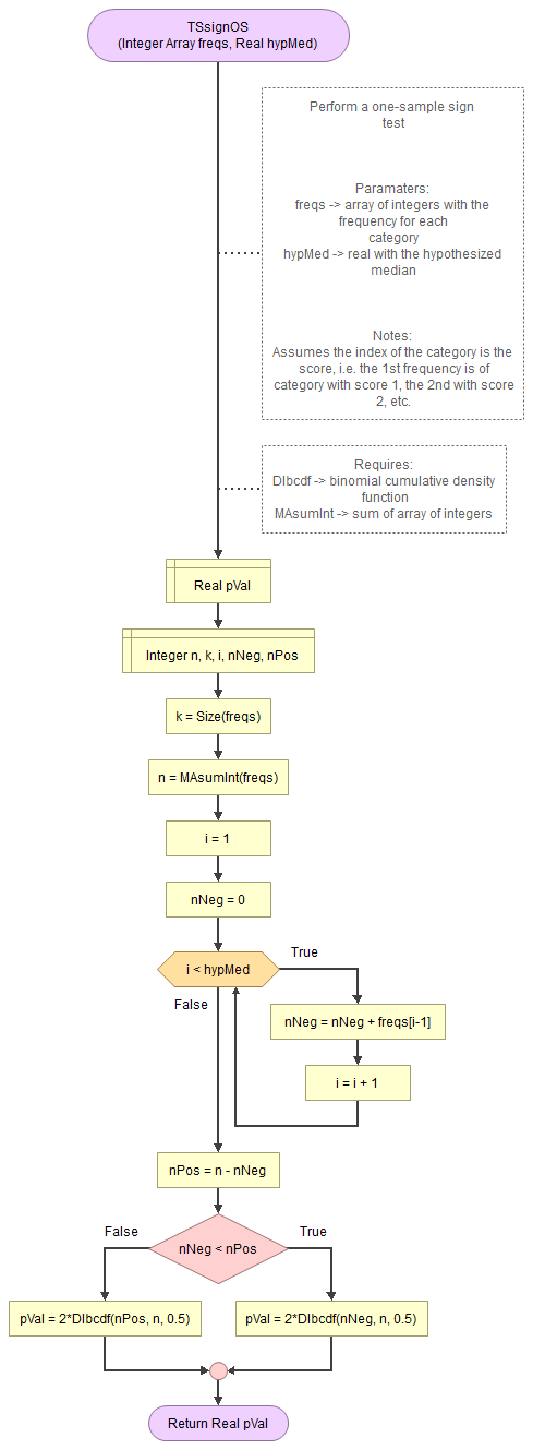
It takes as input an array of integers with the observed frequencies and the hypothesized median.
It uses the function for the binomial cumulative distribution (DIbcdf) and a small helper function to determine the sum of an array. The DIbcdf in turn requires the binomial probability mass function, which in turn uses two helper functions (HEstirlerr and HEbd0). The HEstirlerr function requires the math helper functions factorial and exponential.
Flowgorithm file: FL-TSsignOS.fprg.
with Python
Jupyter Notebook used in video: TS - Sign-test (One-Sample) (P).ipynb.
with stikpetP
without stikpetP
with R
Jupyter Notebook from videos: TS - Sign-test (One-Sample) (R).ipynb.
with stikpetR
without stikpetR
with SPSS
Datafile used in video: GSS2012-Adjusted.sav
Formulas
The one-sample sign test can be performed using:
\(p = 2\times bcdf\left(n, \text{min}\left(n_+, n_-\right), \frac{1}{2}\right) \)
Where \(bcdf\) is the binomial cumulative distribution function, with \(n\) the number of cases used as number of trials, the minimum of \(n_+\) (the number of cases above the hypothesized median) and \(n_-\) (the number of cases below the hypothesized median) as the number of successes, and 0.5 as the probability of success on each trial.
Example
We are given the results of an ordinal variable as a frequency table shown in Table 1.
| Option | Frequency |
|---|---|
| very scientific | 100 |
| pretty scientific | 199 |
| not too scientific | 348 |
| not scientific at all | 307 |
| Total | 954 |
We would like to know if people tended significantly more towards either end. So, as our hypothesized median we set exactly between 'pretty scientific' and 'not too scientific'
The total number of cases is 954 (\(=n\)). The 'very scientific' and 'pretty scientific' are below the hypothesized median, so \(n_- = 100 + 199 = 299\), and the other two categories are above it, so \(n_- = 348 + 307 = 655\)
Filling out these values in the formula to get the significance we get:
\(p = 2\times bcdf\left(954, \text{min}\left(299, 655\right), \frac{1}{2}\right) = 2\times bcdf\left(954, 299, \frac{1}{2}\right) \approx \frac{2.83}{10^{31}} \)
How to calculate a binomial cumulative density function (bcdf) is explained in the binomial distribution section.
The result in the example is far below the usual threshold of 0.05. The population median is therefor significantly different from the hypothesized one. There is a significant tendency to not see accounting as scientific.
Interpreting the Result
The assumption about the population for this test (the null hypothesis) is that the median is a specific value.
The test provides a p-value, which is the probability of a test statistic as from the sample, or even more extreme, if the assumption about the population would be true. If this p-value (significance) is below a pre-defined threshold (the significance level \(\alpha\) ), the assumption about the population is rejected. We then speak of a (statistically) significant result. The threshold is usually set at 0.05. Anything below is then considered low.
If the assumption is rejected, we conclude that the median in the population will be different than the one used in the test.
Note that if we do not reject the assumption, it does not mean we accept it, we simply state that there is insufficient evidence to reject it.
Writing the results
APA (2019) does not specify how to write the results of a one-sample sign test. It shows for most tests to report the test-statistic, the degrees of freedom (if applicable) and the p-value. However with an exact test as the one-sample sign test, there isn't a test-statistic. I would therefor suggest to list the number of scores above and the number of scores below the median and the p-value.
So for example:
A one-sample sign test, indicated that the median was significantly different from the neutral option, n+ = 299, n- = 655, p < .001.
The p-value is shown with three decimal places, and no 0 before the decimal sign. If the p-value is below .0005, it can be reported as p < .001.
APA (2019, p. 88) states to also report an effect size measure.
Google adds