
One-Sample (Student) t-Test
Introduction
The one-sample Student t-test can be used to determine if the mean in a population differs from a pre-defined value, based on a sample. If the sample size is large, the test will produce almost the same results as a one-sample z-test.
Many textbooks will mention that in order to use a t-test the data should be roughly normally distributed. Simplified this means that the histogram should look a bit like a bell-shape. There are tests to check if the data is ‘normal’, but these test if it is normal, not if it is somewhat normal. Lumley, Diehr, Emerson, and Chen (2002) mention that if the sample size is sufficiently large, this criteria to use the test is no longer needed: “previous simulations studies show that “sufficiently large” is often under 100” (p. 166).
The t-test uses the Student t-distribution. Gosset, using his pseudonym Student, is often referred to as the origin for this distribution, who studied it for the Guiness brewery and got an article published it in 1908. However, the distribution was already known, see for example Helmert (1875; 1876a; 1876b) and Lüroth (1876), or in more general form Pearson (1895). Gosset had send his results to Fisher, and Gosset actually used the population variance, which Fisher changed this to the sample variance. Fisher made the test popular by including it in his textbook (1925).
Performing the Test
with Excel
Excel file from video: TS - Student t (one-sample) (E).xlsm
with stikpetE
without stikpetE
with Flowgorithm
A flowgorithm for the one-sample Student t-test in Figure 1.
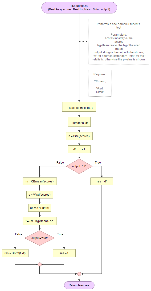
It takes as input the scores, the hypothesized mean, and a string for which output to show (df, statistic, or p-value).
It uses a function for the mean (CEmean), standard deviation (VAsd) and the t cumulative distribution (DItcdf). These in turn require the MAsumReal function (sums an array of real values) and the standard normal cumulative distribution (DIsncdf).
Flowgorithm file: FL-TSstudentOS.fprg.
with Python
Notebook from video: TS - Student t (one-sample) (P).ipynb
with stikpetP
without stikpetP
with SPSS
Formulas
Formula's
The t-value can be determined using:
\(t=\frac{\bar{x}-\mu_{H_{0}}}{SE}\)
In this formula \(\bar{x}\) is the sample mean, \(\mu_{H_0}\) the expected mean in the population (the mean according to the null hypothesis), and SE the standard error.
The standard error can be calculated using:
\(SE=\frac{s}{\sqrt{n}}\)
Where n is the sample size, and s the sample standard deviation.
The formula for the sample standard deviation is:
\(s=\sqrt{\frac{\sum_{i=1}^{n}\left(x_{i}-\bar{x}\right)^{2}}{n-1}}\)
In this formula xi is the i-th score, and n is the sample size.
The sample mean can be calculated using:
\(\bar{x}=\frac{\sum_{i=1}^{n}x_{i}}{n}\)
The degrees of freedom is determined by:
\(df=n-1\)
Where n is the sample size
Example (different example)
We are given the ages of five students, and have an hypothesized population mean of 24. The ages of the students are:
\(X=\left\{18,21,22,19,25\right\}\)
Since there are five students, we can also set n = 5, and the hypothesized population of 24 gives \(\mu_{H_{0}}=24\)
For the standard deviation, we first need to determine the sample mean:
\(\bar{x}=\frac{\sum_{i=1}^{n}x_{i}}{n}=\frac{\sum_{i=1}^{5}x_{i}}{5}=\frac{18+21+22+19+25}{5}\)
\(=\frac{105}{5}=21\)
Then we can determine the standard deviation:
\(s=\sqrt{\frac{\sum_{i=1}^{n}\left(x_{i}-\bar{x}\right)^{2}}{n-1}}=\sqrt{\frac{\sum_{i=1}^{5}\left(x_{i}-21\right)^{2}}{5-1}}=\sqrt{\frac{\sum_{i=1}^{5}\left(x_{i}-21\right)^{2}}{4}}\)
\(=\sqrt{\frac{\left(18-21\right)^{2}}{4}+\frac{\left(21-21\right)^{2}}{4}+\frac{\left(22-21\right)^{2}}{4}+\frac{\left(19-21\right)^{2}}{4}+\frac{\left(25-21\right)^{2}}{4}}\)
\(=\sqrt{\frac{\left(-3\right)^{2}}{4}+\frac{\left(0\right)^{2}}{4}+\frac{\left(1\right)^{2}}{4}+\frac{\left(-2\right)^{2}}{4}+\frac{\left(4\right)^{2}}{4}}\)
\(=\sqrt{\frac{9}{4}+\frac{0}{4}+\frac{1}{4}+\frac{4}{4}+\frac{16}{4}}=\sqrt{\frac{9+0+1+4+16}{4}}=\sqrt{\frac{30}{4}}\)
\(=\sqrt{\frac{15}{2}}=\frac{1}{2}\sqrt{15\times2}=\frac{1}{2}\sqrt{30}\approx2.74\)
The standard error then becomes:
\(SE=\frac{s}{\sqrt{n}}=\frac{\frac{1}{2}\sqrt{30}}{\sqrt{5}}=\frac{\frac{\sqrt{30}}{2}}{\sqrt{5}}=\frac{\sqrt{30}}{2\times\sqrt{5}}\)
\(=\frac{1}{2}\times\frac{\sqrt{30}}{\sqrt{5}}=\frac{1}{2}\times\sqrt\frac{30}{5}=\frac{1}{2}\sqrt{6}\approx1.22\)
The t-value:
\(t=\frac{\bar{x}-\mu_{H_{0}}}{SE}=\frac{21-24}{\frac{1}{2}\sqrt{6}}=\frac{-3}{\frac{\sqrt{6}}{2}}=\frac{-3\times2}{\sqrt{6}}=\frac{-6}{\sqrt{6}}\)
\(gif.latex?=\frac{-6}{\sqrt{6}}\times\frac{\sqrt{6}}{\sqrt{6}}=\frac{-6\times\sqrt{6}}{\sqrt{6}\times\sqrt{6}}=\frac{-6\times\sqrt{6}}{6}=-\sqrt{6}\approx-2.45\)
The degrees of freedom is relatively simple:
\(df=n-1=5-1=4\)
The two-sided significance is then usually found by using the t-value and the df, and consulting a t-distribution table, or using some software. If you really had to determine it manually, it would involve the formula for the t-distribution (the cumulative density function):
\(2\times\int_{x=|t|}^{\infty}\frac{\Gamma\left(\frac{df+1}{2}\right)}{\sqrt{df\times\pi}\times\Gamma\left(\frac{df}{2}\right)}\times\left(1+\frac{x^2}{df}\right)^{-\frac{df+1}{2}}\)
See the Student t-distribution section for more details.
Interpreting the Result
The assumption about the population for this test (the null hypothesis) is that the mean is a specific value.
The test provides a p-value, which is the probability of a test statistic as from the sample, or even more extreme, if the assumption about the population would be true. If this p-value (significance) is below a pre-defined threshold (the significance level \(\alpha\) ), the assumption about the population is rejected. We then speak of a (statistically) significant result. The threshold is usually set at 0.05. Anything below is then considered low.
If the assumption is rejected, we conclude that the mean in the population will be different than the one used in the test.
Note that if we do not reject the assumption, it does not mean we accept it, we simply state that there is insufficient evidence to reject it.
Writing the results
Writing up the results of the test uses the format (APA, 2019 p. 182):
t(<degrees of freedom.>) = <t-value>, p = <p-value>
So for example:
The mean age of customers was 48.19 years (SD = 17.69). The claim that the average age is 50 years old can be rejected, t(1968) = -4.53, p < .001.
The p-value is shown with three decimal places, and no 0 before the decimal sign. If the p-value is below .0005, it can be reported as p < .001. The abbreviation of 'SD' for standard deviation, is not needed to be explained, it is an accepted abbreviation in APA (2019, p. 185).
APA (2019, p. 88) states to also report an effect size measure.
Google adds