
Mean
Explanation
Three means are referred to as the Pythagoras means: the arithmetic, harmonic, and geometric mean. These can be seen from a geometric perspective as illustrated in figure 1.
Figure 1Pythagoras Means from Geometry Perspective
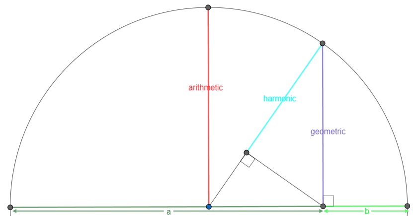
The arithmetic mean is what most people will consider as 'the' mean, and is often the one referred to as the average (although average could refer to any measure of central tendency so also for example the mode or median). Ask someone what the mean (or average) is, and most often you will hear the calculation: the sum divided by the number of items. However this explains how to calculate it, not what it conceptually actually means. One conceptual definition is “the fulcrum that is unique to each distribution” (Weinberger & Schumacher as cited in Watier, Lamontagne, & Chartier, 2011, p. 3). A fulcrum is the balancing points. To illustrate this, the animated gif in figure 2 shows an example.
Figure 2Arithmetic mean as fulcrum
The arithmetic mean is also sometimes seen as the most 'social'. It shows the value that everyone would get, if everyone would get the same amount.
The harmonic mean is often used with ratios. It can for example show the average speed of a round trip, if the speed one-way was different than the other. The harmonic mean gives a lot of weight to small numbers, and could be useful if you have some extreme high values.
The geometric mean is often used with compound interest. If in year one you have a 1.05 (so a 5% interest) growth rate, in year 2 a 1.02 and in year 3 a 1.07, then the geometric mean will give you a growth rate of appr. 1.0465, indicating we could have used an interest rate of 4.645% for each year.
Since extreme values can have a big impact on the mean, many have derived methods to avoid including the extreme values in the calculations. These are:
- trimmed, truncated, or Windsor mean, remove the highest and lowest x% of scores
- Winsorized mean, replace the highest and lowest x% of scores with closest value not being replaced
- olympic mean, simply remove the maximum and minimum, then use arithmetic mean on remaining scores
- decile mean, determine the 9 deciles (quantiles with 10% to 90%) and determine the arithmetic mean from these nine
Another measure is the mid-range, which is simply the average of the maximum and minimum. This is of course very quickly influenced by extreme values, so often instead the mid-quartile range is used, the average of the first and third quartile. The mid-quartile range is discussed on the quartile ranges page.
Obtaining the Measures
with Python
Notebook from video: ME - Means (P).ipynb
using stikpetP
with other libraries
without libraries
with SPSS
Formula
Arithmetic Mean
The formula (see for example Aristotle (384-322 BC) (1850, p. 43)):
\(\bar{x} = \frac{\sum_{i=1}^n x_i}{n}\)
Harmonic Mean
\(H = \frac{n}{\sum_{i=1}^n \frac{1}{x_i}}\)
Geometric Mean
\(G = e^{\frac{1}{n}\times\sum_{i=1}^n \ln\left(x_i\right)}\)
Olympic Mean
Simply ignore the maximum and minimum (only once) (Louis et al., 2023, p. 117):
\(OM = \frac{\sum_{i=2}^{n-1} x_i}{n - 2}\)
Mid Range
The average of the maximum and minimum (Lovitt & Holtzclaw, 1931, p. 91):
\(MR = \frac{\min x + \max x}{2}\)
Trimmed
With a trimmed (Windsor/Truncated) mean we trim a fixed amount of scores from each side (Tukey, 1962, p. 17). Let \(p_t\) be the proportion to trim, we then need to trim \(n_t = \frac{p_t\times n}{2}\) from each side.
If this \(n_t\) is an integer there isn't a problem, but if it isn't we have options. The first option is to simply round down, i.e. \(n_l = \lfloor n_t\rfloor\). The trimmed mean is then:
\(\bar{x}_t = \frac{\sum_{i=n_t+1}^{n - n_l + 1} x_i}{n - 2\times n_l}\)
We could also use linear interpolation based on the number of scores to trim. We missed out on: \(f = n_t - n_l\) on each side. So the first and last value we do include should only count for \(1 - f\) each. The trimmed mean will then be:
\(\bar{x}_t = \frac{\left(x_{n_t + 1} + x_{n - n_l + 1}\right)\times\left(1 - f\right) + \sum_{i=n_l+2}^{n - n_l} x_i}{n - 2\times n_t}\)
Alternative, we could take the proportion itself and use linear interpolation on that. The found \(n_l\) will be \(p_1 = \frac{n_l \times 2}{n}\) of the the total sample size. While if we had rounded up, we had used \(p_2 = \frac{\left(n_l + 1\right)\times 2}{n}\) of the the total sample size. Using linear interpolation we then get:
$$\bar{x}_t = \frac{p_t - p_1}{p_2 - p_1}\times\left(\bar{x}_{th}-\bar{x}_{tl}\right) + \bar{x}_{tl}$$
Where \(\bar{x}_{tl}\) is the trimmed mean if \(p_1\) would be used as a trim proportion, and \(\bar{x}_{th}\) is the trimmed mean if \(p_2\) would be used.
Note: the term Windsor mean is for example used by Wenzl (2016, p. 65)
Winsorized Mean
Similar as with a trimmed mean, but now the data is not removed, but replaced by the value equal to the nearest value that is still included (Winsor as cited in Dixon, 1960, p. 385).
$$W = \frac{n_l \times \left(x_{n_l + 1} + x_{n - n_l}\right) + \sum_{n_l + 1}^{n - n_l} x_i}{n}$$
Decile Mean
The formula used is (Rana et al., 2012, p. 480)
$$DM = \frac{\sum_{i=1}^k D_i}{9}$$
Where \(D_i\) is the i-th decile score (quantiles with k=10).
Google adds