
Binning
Binning is to place scores into bins. It is often done with a scale variable. When creating bins two important rules should be followed:
- the bins should not overlap.
- each score should fit into a bin.
These two rules, can be combined into one: each score should fit into exactly one bin.
Deciding on the number of bins, is probably the most difficult. Too few bins, and you loose too much information; too many and you loose the overview. The easiest method is probably to simply use a rule of thumb, such as between 5 and 15 bins (Herkenhoff & Fogli, 2013, p. 58), but different methods exist for this. More information on number of bins in its own section below.
Notation is another issue, and is discussed in it's own section below.
Click here to see how you can create bins...
with Excel
The Data Analysis Toolkit that comes with Excel could be used to create the bins, but those bins will then include the upper bound. It is also possible to do it without the toolkit.
without the Data Analysis Toolkit
Excel file: IM - Binning.xlsm.
with the Data Analysis Toolkit
Excel file: IM - Binning.xlsm.
with Python
Jupyter Notebook used in video: IM - Binning (Create).ipynb.
Data file used: GSS2012a.csv.
with R (Studio)
Jupyter Notebook: IM - Binning (Create) (R).ipynb
R script: IM - Binning (create).R.
Data file used: GSS2012a.csv.
with SPSS
Data file used: Holiday Fair.sav.
Click on a section below to reveal its content.
Number of Bins
The number of bins can have quite an impact on how the results look. In figure 1 four different number of bins were used and compared.
Figure 1.
Example of different number of bins
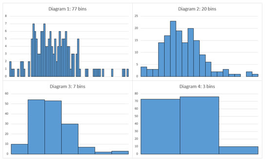
In diagram 1 it is very hard to see any pattern, as well as in diagram 4. Diagram 2 would show a rise to a peak, a small drop and then another smaller peak. In diagram 3 there is only one peak. When binning numerical data into bins the question about the number of bins (k) comes up or similarly the bin size (h). There are quite a lot of different methods to determine this and to my knowledge no single agreed upon method has yet been developed. In a comparison among 42 introductory statistics textbooks (done by myself) the square root choice (Duda & Hart, 1973) was only mentioned three times, Sturges' rule (Sturges, 1926, p. 65) twice and Kelley's rule only in his own textbook. There were 28 textbooks giving some guideline on the number of bins (12 x '5 to 20', 10 x '5 to 15', 3 x '10 to 20', and the following each once '4 to 20', '5 to 10', '6 to 15'), two textbooks simply mentioned 'around 10', and six did not have any clear guideline.
An interesting overview is available in the dissertation of Lohaka (2007). SPSS uses quite sophisticated procedures from Fayyad and Irani (1993), Dougherty, Kohavi, and Sahami (1995) and Liu et al. (2002).
Click here to see how you to determine the number of bins...
with R (Studio)
Notebook from video: IM - Binning (nr of bins) (R).ipynb
with stikpetR:
without stikpetR:
manually (formula's)
For the formula's below \(k\) is the number of bins, and \(n\) the sample size. The \(\left \lceil \dots \right \rceil\) is the ceiling function, which means to round up to the nearest integer
Square-Root Choice (Duda & Hart, 1973)
\( k = \left \lceil\sqrt{n}\right \rceil \)
Sturges (1926, p. 65)
\( k = \left\lceil\log_2\left(n\right)\right\rceil+1 \)
QuadRoot (anonymous as cited in Lohaka, 2007, p. 87)
\( k = 2.5\times\sqrt[4]{n} \)
Rice (Lane, n.d.)
\( k = \left\lceil 2\times\sqrt[3]{n} \right\rceil \)
Terrell and Scott (1985, p. 209)
\( k = \sqrt[3]{2\times n} \)
Exponential(Iman & Conover as cited in Lohaka, 2007, p. 87)
\( k = \left\lceil\log_2\left(n\right)\right\rceil \)
Velleman (Velleman, 1976 as cited in Lohaka 2007)
\( \begin{cases}2\times\sqrt{n} & \text{ if } n\leq 100 \\ 10\times\log_{10}\left(n\right) & \text{ if } n > 100\end{cases} \)
Doane(1976, p. 182)
\( k = 1 + \log_2\left(n\right) + \log_2\left(1+\frac{\left|g_1\right|}{\sigma_{g_1}}\right) \)
In the formula's \(g_1\) the 3rd moment skewness:
\( g_1 = \frac{\sum_{i=1}^n\left(x_i-\bar{x}\right)^3} {n\times\sigma^3} = \frac{1}{n}\times\sum_{i=1}^n\left(\frac{x_i-\bar{x}}{\sigma}\right)^3 \)
With \(\sigma = \sqrt{\frac{\sum_{i=1}^n\left(x_i-\bar{x}\right)^2}{n}}\)
The \(\sigma_{g_1}\) is defined using the formula:
\( \sigma_{g_1}=\sqrt{\frac{6\times\left(n-2\right)}{\left(n+1\right)\left(n+3\right)}} \)
Formula's that determine the width (h) for the bins
Using the width and the range, it can be used to determine the number of categories:
\( k = \frac{\text{max}\left(x\right)-\text{min}\left(x\right)}{h} \)
Scott (1979, p. 608)
\( h = \frac{3.49\times s}{\sqrt[3]{n}} \)
Where \(s\) is the sample standard deviation:
\(s = \sqrt{\frac{\sum_{i=1}^n\left(x_i-\bar{x}\right)^2}{n-1}}\)
Freedman-Diaconis (1981, p. 3)
\( h = 2\times\frac{\text{IQR}\left(x\right)}{\sqrt[3]{n}} \)
Where \( \text{IQR}\) the inter-quartile range.
A more complex technique is for example from Shimazaki and Shinomoto (2007). For this, we define a 'cost function' that needs to be minimized:
\( C_k = \frac{2\times\bar{f_k}-\sigma_{f_k}}{h^2} \)
With \(\bar{f_k}\) being the average of the frequencies when using \(k\) bins, and \(\sigma_{f_k}\) the population variance. In formula notation:
\(\bar{f_k}=\frac{\sum_{i=1}^k f_{i,k}}{k}\)
\(\sigma_{f_k}=\frac{\sum_{i=1}^k\left(f_{i,k}-\bar{f_k}\right)^2}{k}\)
Where \(f_{i,k}\) is the frequency of the i-th bin when using k bins.
Note that if the data are integers, it is recommended to use also bin widths that are integers.
Stone (1984, p. 3) is similar, but uses as a cost function:
\(C_k = \frac{1}{h}\times\left(\frac{2}{n-1}-\frac{n+1}{n-1}\times\sum_{i=1}^k\left(\frac{f_i}{n}\right)^2\right)\)
Knuth (2019, p. 8) suggest to use the k-value that maximizes:
\(P_k=n\times\ln\left(k\right) + \ln\Gamma\left(\frac{k}{2}\right) - k\times\ln\Gamma\left(\frac{1}{2}\right) - \ln\Gamma\left(n+\frac{k}{2}\right) + \sum_{i=1}^k\ln\Gamma\left(f_i+\frac{1}{2}\right)\)
Symbols
The range of the bin could include or exclude each of the two bounds. Often it is assumed that the lower bound is included, and then either less than (<) is used to exclude the upper bound, or less than or equal to (≤) to include the upper bound.
You might also encounter a symple hyphen (-), but this could mean to exclude the upper bound (Sharma, Kumar, & Chaudhary, 2009, p. 31), or to include it (Haighton, Haworth, & Wake, 2003, p. 24). I wouldn't recommend using it.
More technical is the use of square brackets ([ and ]) to indicate included bounds, and parenthesis (( and )), to indicate excluded, or a combination. This allows to also exclude the lower bound. For example (5, 8] would exclude 5 and include 8.

Google adds