t-Distribution

Gosset, using his pseudonym Student, is often referred to as the origin for this distribution, who studied it for the Guiness brewery and got an article published it in 1908. However, the distribution was already known, see for example Helmert (1875; 1876a; 1876b) and Lüroth (1876), or in more general form Pearson (1895).

The distribution is very similar to the standard normal distribution, it also looks like a bell-shape, is continuous, and is symmetrical. The t-distribution is a bit lower and wider, but if the sample size increases it becomes almost identical to the normal distribution as illustrated in figure 1.

Figure 1
t to normal approximation

Note that the peak of the curve is always at the mean, and the higher the standard deviation, the 'flatter' the bell looks.

As with any continuous distribution it is very important to remember that we are usually only interested in the areas under the curve, since those give us the probability

Now calculating this area can be tricky business depending on how easy you want to make it on yourself

Use some software (easy)

Excel

TO BE UPLOADED

Python

TO BE UPLOADED

SPSS

TO BE UPLOADED

Use tables (old school)

In figure 2 an example of a Student t-distribution right-tail table, with critical t-values.

Figure 2
Student t-distribution right-tail table"

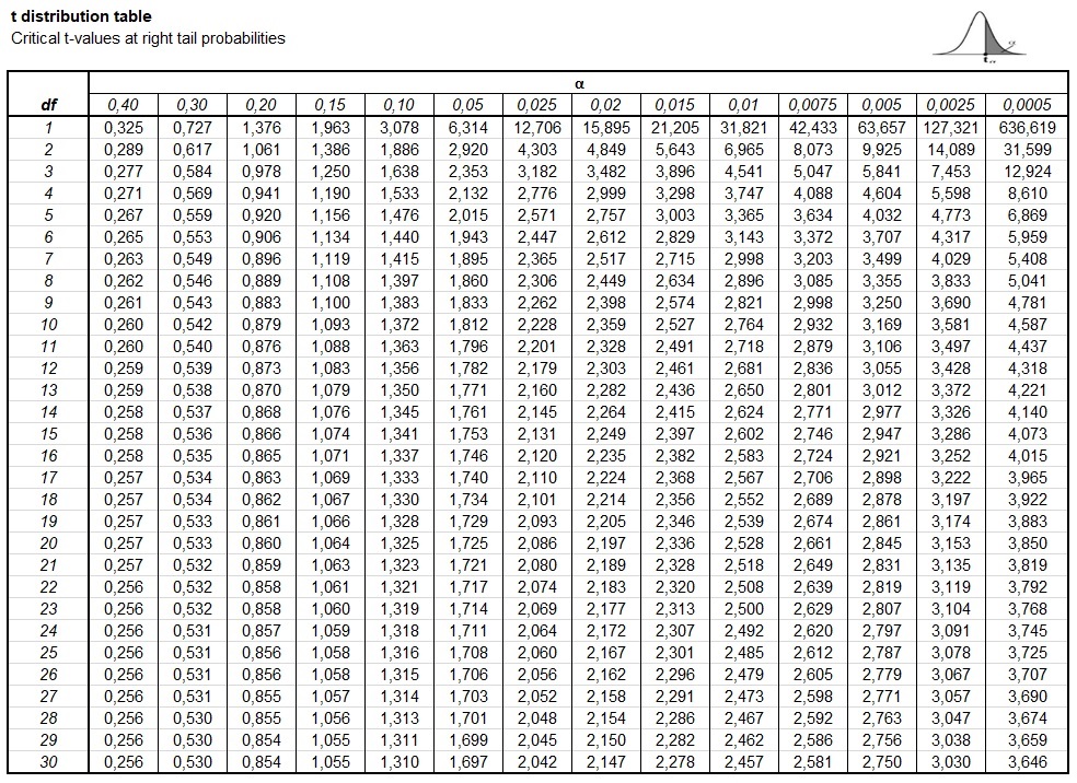
This table will show the critical t-value at a chosen degrees of freedom, and alpha. WARNING: this shows the right-tail probability. So if we want to know if something is significant at the 95% level, we do the following. The alpha level is 0.05, but since the table only shows the right-tail, for the table we use this alpha level divided by 2. In this example that would be 0.025.

If our degrees of freedom is for example 8, and we want 95% confidence, then the critical t-value is found 2.306. It's a the intersection of the row of df=8 and the column of alpha=0.025.

If the t-value we calculate is higher than this critical t-value, we would consider it significant.

Alternative, if we have the t-value we calculated, we can look where it appears in the row of the degrees of freedom. Usually the exact value will not be there, so it will fall between two values. For example if we have a t-value of 1.9 and still a degrees of freedom of 8, the 1.9 falls between the 1.860 and 2.306. These two values correspond to the columns 0.05 and 0.025.

Remember though, that this is the right-tail only. So for a two-sided test we simply multiply each to get 0.05×2 = 0.1 and 0.025×2=0.05. We could then conclude that the p-value would be between 0.05 and 0.1.

We could use linear interpolation to approximate the p-value. We have a total width of 2.306 - 1.86 = 0.446. Our t-value of 1.9 is from the start 1.9 - 1.86 = 0.04, so a total of 0.04 / 0.446 = 8.97%. Now from the p-values we have a total width of 0.05 - 0.1 = -0.5. If we take 8.97% from this, we get -0.004. We add this to the lower amount and get 0.1 + -0.004 = 0.096. This calculation is visualised in figure 3

Figure 3
Example of t-distribution table interpolation
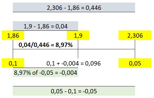The exact p-value of a t-value of 1.9 and degrees of freedom 8 would have been 0.094, so it was quite close.

Do the math (hard core)

The probability density function (the curves shown in figure 1) has the following equation:

\(tpdf\left(t, df\right) = \frac{\Gamma\left(\frac{df+1}{2}\right)}{\sqrt{df\times\pi}\times\Gamma\left(\frac{df}{2}\right)} \times \left(1+\frac{t^2}{df}\right)^{-\frac{df+1}{2}}\)

In this equation \(df\) is the degrees of freedom, and \(t\) the t-value. The \(\Gamma\) is the gamma function

The gamma function appears twice in the equation, but each with df, which should usually be an integer, if df is an integer we can define the gamma function as:

\( \Gamma\left(a=\frac{x}{2}\right)=\begin{cases} \left(a - 1\right)! & \text{ if } x \text{ is even}\\ \frac{\left(2\times a\right)!}{4^a\times a!}\times\sqrt{\pi} & \text{ if } x \text{ is odd} \end{cases} \)

The cumulative density function is 'simply' the integral of the pdf:

\(tcdf\left(t, df\right)= \int_{u=-\infty}^{t}tpdf\left(u,df\right)du\)

It can also be written with a so-called incomplete beta function:

\(tcdf\left(t, df\right)= 1-\frac{1}{2}\times I_{x\left(t\right)}\left(\frac{df}{2},\frac{1}{2}\right)\)

With \(x\left(t\right)=\frac{df}{t^2+df}\)

The \(I\) indicates the regularized incomplete beta function and can be defined as (DLMF eq. 8.17.2):

\(I_x\left(a,b\right) = \frac{B\left(x;a,b\right)}{B\left(a,b\right)}\)

In this fraction the numerator is the incomplete beta function and the denominator the complete beta function.

The complete beta function can be expressed with the gamma function (DLMF eq. 5.12.1):

\(B\left(x,y\right) = \frac{\Gamma\left(x\right)\times\Gamma\left(y\right)}{\Gamma\left(x+y\right)}\)

The gamma function has already been discussed above. The problem is the incomplete beta function, which can be expressed as (DLMF eq. 8.17.7):

\(B\left(x;a,b\right) = \frac{x^a}{a}\times F\left(a, 1 - b;a+1;x\right)\)

Where \(F\left(a, b;c ; z\right)\) is the hypergeometric function (DLMF eq. 15.2.1).

\(F\left(a,b;c;z\right)=\sum_{s=0}^{\infty}\frac{{\left(a\right)_{s}}{\left(b% \right)_{s}}}{{\left(c\right)_{s}}s!}z^{s}=\frac{\Gamma\left(c\right)}{\Gamma\left(a\right)\Gamma% \left(b\right)}\sum_{s=0}^{\infty}\frac{\Gamma\left(a+s\right)\Gamma\left(b+s% \right)}{\Gamma\left(c+s\right)s!}z^{s}\)

Calculating this is beyond the scope of this site, instead two alternatives...

use bars to approximate

to be added...

algorithms

Dudewicz and Dalal

According to Dudewicz and Dalal (1972) the cdf can also be described with the following set of rules:

If \(df=1\):

\(tcdf\left(t, df\right) = \frac{1}{2} + \frac{\theta}{\pi}\)

If \(df>1\text{ and }df=odd\):

\(tcdf\left(t, df\right) = \frac{1}{2} + \frac{1}{\pi}\left(\theta + \sin\theta \times \left(\cos\theta + \sum_{i=1}^{\frac{df-3}{2}} \cos^{i\times2+1}\theta\times \prod_{j=1}^{i}\frac{j\times 2}{j\times 2 + 1} \right)\right)\)

If \(df=even\):

\(tcdf\left(t, df\right) = \frac{1}{2}+\frac{\sin \theta}{2}\left(1 + \sum_{i=1}^{\frac{df}{2}}\cos^{i*2}\theta \prod_{j=1}^{i} \frac{j\times2 - 1}{j\times2}\right)\)

ACM Algorithm 395

Hill (1970, 1981) developed an algorithm ACM 395. It uses the standard normal approximation in extreme cases. Figure 2 shows a flow chart of the algorithm.

Figure 2
ACM Algorithm 395 flow chart

Using adjusted Normal approximation

Since the t-distribution has a lot of similarities with the standard normal distribution, many have come up with adjustments of the standard normal distribution to approximate the t-distribution.

Gaver and Kafadar (1984, p. 309) proposed:

\(A_1 = tcdf\left(t, df\right) \approx sncdf\left(z_1\right)\)

Where \(sncdf\) is the standard normal cumulative distribution function and:

\(z_1 = \sqrt{\frac{\ln\left(1+\frac{t^2}{df}\right)}{g_1}}\)

and

\(g_1=\frac{df-1.5}{\left(df-1\right)^2}\)

Gleason (2000, p. 64) improved on Gaver and Kafadar for small values of df.

\(A_2 = tcdf\left(t, df\right) \approx sncdf\left(z_2\right)\)

Where \(sncdf\) is the standard normal cumulative distribution function and:

\(z_2 = \sqrt{\frac{\ln\left(1+\frac{t^2}{df}\right)}{g_2}}\)

and

\(g_2=\frac{df-1.5-\frac{0.1}{df}+\frac{0.5825}{df^2}}{\left(df-1\right)^2}\)

Boiroju and Kumar (2014, p. 109) improved further on the version from Gleason (2000) and suggest:

\(A_3 = tcdf\left(t, df\right) \approx A_2 - \frac{7.9+7.9\times\text{tanh}\left(3-0.63\times x - 0.52\times df\right)}{10000}\)

Where \(A_2\) is the approximation from Gleason and

\(x = \begin{cases} 9 & \text{ if } t=0\\ t & \text{ otherwise }\end{cases}\)

Li and De Moor (1999) proposed:

\(A_4 = tcdf\left(t, df\right) \approx \begin{cases} \frac{1}{2} + \frac{1}{\pi}\times atan\left(t\right) & \text{ if } df=0 \\ \frac{1}{2} + \frac{t}{2}\times\left(2+t^2\right)^{-\frac{1}{2}} & \text{ if } df=2 \\ sncdf\left(t\times\frac{4\times df+t^2-1}{4\times df + 2\times t^2}\right) & \text{otherwise}\end{cases}\)

Where \(sncdf\) is the standard normal cumulative distribution function

Boiroju and Kumar (2014, p. 109) also made a decision tree style approximation using the previous three (their own, Gleason and Li & De Moor):

\(A_5 = tcdf\left(t, df\right) \approx \begin{cases} A_4 & \text{ if } t < 1.3+0.04\times df \\ A_3 & \text{ if } 1.3+0.04\times df \le t < 5.94-0.04\times df \\ A_2 & \text{otherwise}\end{cases}\)

Where \(A_2\) is the approximation from Gleason, \(A_3\) the approximation from Boiroju and Kumar, and \(A_4\) the approximation from Li and De Moor.

Numerical Approximation

Gentleman and Jenkins (1968) made a numerical approximation, but only for df > 5. They define the following values:

Table 1
Values for a
i	a_i0	a_i1	a_i2	a_i3	a_i4
1	0.09979441	-0.581821	1.390993	-1.222452	2.151185
2	0.04431742	-0.2206018	-0.03317253	5.679969	-12.96519
3	0.009694901	-0.1408854	1.88993	-12.75532	25.77532
4	-0.00009187228	0.03789901	-1.280346	9.249528	-19.08115
5	0.00579602	-0.02763334	0.4517029	-2.657697	5.127212

Table 2
Values for b
i	b_i1	b_i2
1	-5.537409	11.42343
2	-5.166733	13.49862
3	-4.233736	14.3963
4	-2.777816	16.46132
5	-0.5657187	21.23269

For the coefficients the following formula is used:

\(c_i = \frac{\sum_{j=0}^4 a_{ij}\times df^{-i}}{\sum_{k=0}^2 b_{ik}\times df^{-k}} = \frac{a_{i0} + a_{i1}\times df^{-1} + a_{i2}\times df^{-2} + a_{i3}\times df^{-3} + a_{i4}\times df^{-4}}{1 + b_{i1}\times df^{-1} + b_{i2}\times df^{-2}}\)

To approximate the t-cumulative distribution function:

\(tcdf\left(t, df\right) \approx 1 - \left(1 + \sum_{i=1}^5 c_i\times t^i\right)^{-8}\)

Links to parts

Google adds