
Mann-Whitney(-Wilcoxon Rank Sum) Distribution
The exact distribution of the Mann-Whitney(-Wilcoxon) U statistic (or Wilcoxon Rank Sum) is a bit tricky. It is created by having two independent samples, each with a sample size. So for example if we have scores on something from 'national' companies and 'international'companies.
The MWW-distribution will show us in general if we have \(n_1\) cases in one category and \(n_2\) in the other, how often we can get a specific \(U\) value. So for example a sum of ranks of 7 for the category with 3 options would only be possible with the 1, 2, 4. However a sum of 8 would have been possible with 1-2-5, or with 1-3-4. The \(U\) value is the sum of ranks minus the minimum possible sum of ranks. Figure 1 shows some distributions for variuous combinations of \(n_1\) and \(n_2\).
Figure 1
Mann-Whitney U Distribution Examples

The distribution quickly starts to look like a normal distribution, which is why very often a normal approximation is used, rather than the exact test.
Use a distribution table (old school)
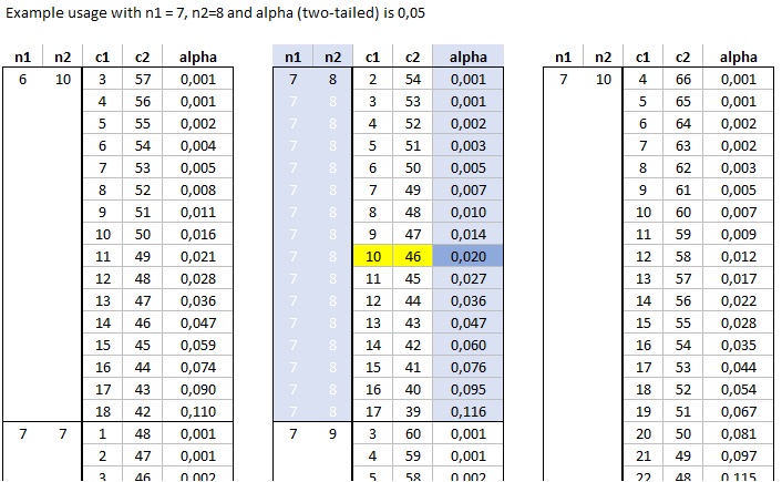
In figure 2 a table with critical U values is shown.
Figure 2
Cumulative Binomial Distribution Table - Version 1a
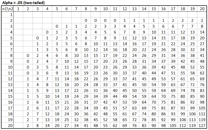
The table shown above shows till which \(U\) value the cumulative probability multiplied by two (since it is a two-tailed table), will still be below the alpha level of .05, for various combinations of sample sizes \(n_1\) and \(n_2\). For example, if we had a sample size of 7 in the first category and 8 in the second, any U value below or equal to 10, would result in a two-sided p-value less than 0.05.
Note that the maximum rank would be \(n_1\times n_2 = 7\times 8 = 56\), and since the distribution is symmetrical, any U value above \(56 - 10 = 46\) would also be critical.
This version of the tables only shows the lowest option. Another issue is that it actually has the same information twice since the critical value for a combination of 7 and 8 cases, is the same as that for 8 and 7 cases. Lastly, this variation requires multiple tables, one for each possible alpha. A few of these can be found on the website Real Statistics Using Excel.
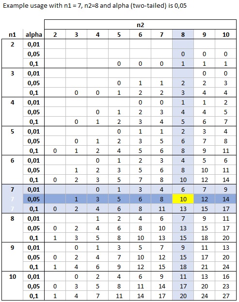
To avoid multiple tables, a variation as shown in Figure 4 is sometimes used.
Figure 4
Cumulative Binomial Distribution Table - Version 1b

With this variation, we again look in the n1-n2 combination of interest (in the example 7 and 8), and now look in the appropriate row of the three possible alpha (two-sided) values. Again we find the critical U value of 10. The process is illustrated in Figure 5.
Figure 5
Cumulative Binomial Distribution Table - Version 1b - Example Usage
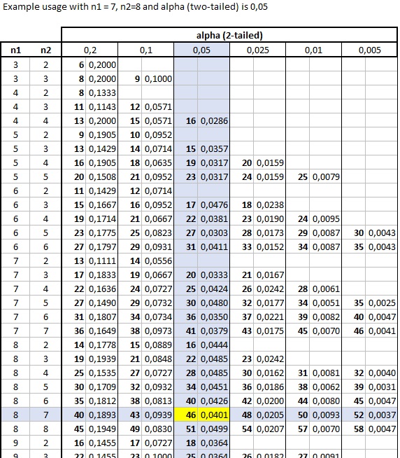
Another variation on the tables is shown in Figure 6. This variation can be found in (Samuels et al., 2012, p. 623).
Figure 6
Cumulative Binomial Distribution Table - Version 2

If we have 7 cases in the first category and 8 in the second, we can simply look at the result for 8 in the first and 7 in the second, since these would be the same. Then at the intersection with an alpha of 0.05 column, we find a U value in bold of 46, which corresponds to a p-value of 0.0401. Unlike the previous version, this is the upper-criteria, as in any U value of 46 or more would be significant at a 0.05 alpha level. To get the lower-criteria we need to subtract the maximum possible U from this, which is \(n_1\times n_2\), so we get \(7\times 8 - 46 = 56 - 46 = 10\). Similar as we found in version 1 tables, a U value of 10 or less would also be significant. The process is illustrated in Figure 7.
Figure 7
Cumulative Binomial Distribution Table - Version 2 - Example Usage
A third variation is found in Statistical tables and formulae (Kokoska & Nevison, 1992, pp. 77-80). They actually show tables for the Wilcoxon Rank Sum statistic, but by subtracting the minimum sum of ranks, these can easily be converted to tables for the U-statistic. Part of the tables is shown in figure 8.
Figure 8
Cumulative Binomial Distribution Table - Version 3
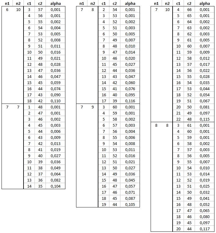
In the image above, the values are already converted for the U-statistic.
If we have 7 cases in the first category and 8 in the second, we can look in the section of n1=7 and n2=8. We now look in the alpha column. This is the one-sided alpha, so if we have a two-tailed test with alpha = 0.05, we look for the one-sided alpha of 0.05/2 = 0.025. We need to find the closest value that is less than or equal to this. In the example this is at 0.020. The c1 and c2 show the lower U value and upper U value resp. So for example a U value of 10 or less, and a U value of 46 or more, each have a probability of 0.02. Together (i.e. two-sided) this becomes 0.04. The process is illustrated in Figure 9.
Figure 9
Cumulative Binomial Distribution Table - Version 3 - Example Usage
The advantage of this version of the table is that it has the p-values for various U values, always showing all possible U's with alpha value between 0.001 and 0.1. The downside is of course that this creates much more 'tables'.
Use the formulas (hard core)
A formula for the count of the Mann-Whitney U distribution is given by a recursive formula:
\(f_{n_1, n_2}(U) = \begin{cases} 0 & \text{ if } U < 0 \text{ or } U > n_1\times n_2 \\ 1 & \text{ if } (n_1=1 \text{ or } n_2=1) \text{ and } 0 \leq U \leq n_1\times n_2 \\ f_{n_1, n_2-1}(U) + f_{n_1-1, n_2}(U - n_2) & \text{ else } \end{cases} \)
This formula is found in Mann and Whitney (1947, p. 51), Dinneen and Blakesley (1973, p. 269) and described also in Festinger (1946).
The total number of combinations, is given by the binomial coefficient:
\(C(n, n_1) = nCr(n, n_1) = \binom{n}{n_1} = \frac{n!}{n_1!\times\left(n - n_1\right)!}\)
with \(n=n_1+n_2\).
The probability mass function can then be written as:
\(pmf_{n_1, n_2-1}(U) = \frac{f_{n_1, n_2}(U)}{\binom{n_1+n_2}{n_1}}\)
The cumulative density function is then:
\(cdf_{n_1, n_2-1}(U) = \sum_{i=0}^U pmf_{n_1, n_2-1}(i)\)
There are also methods by Harris and Hardin (2013) and by Löffler (1983) but I couldn't get those to work.
Worked Out Example
Let's say we have a sample size of 4 in our first category and 3 in the second, i.e. \(n_1 = 4, n_2=3\). We also have a U-statistic of 5.
The U value is the sum of the ranks, minus the minimum possible sum. With 4 cases out of 4+3=7, the minimum would be the sum of the four lowest ranks, i.e. 1+2+3+4 = 10. If we add this to the requested U value of 5, we were looking for the number of ways to get a sum of 15, with four ranks.
These could be 1+2+5+7, 1+3+4+7, 1+3+5+6, 2+3+4+6, so only four options. We could simply each time try to find all the possible combinations, but the recursive function will do the same.
Let's go over all the steps. We begin with filling out our values
\(f_{4, 3}(5) = f_{4, 3-1}(5) + f_{4-1, 3}(5 - 3)= f_{4, 2}(5) + f_{3, 3}(2)\)
Lets focus on the last term each time. First \(f_{3, 3}(2)\), we can use the formula again:
\(f_{3, 3}(2) = f_{3, 3-1}(2) + f_{3-1, 3}(2 - 3)= f_{3, 2}(2) + f_{2, 3}(-1)\)
For \(f_{2, 3}(-1)\) we can use the first case since U < 0, we get
\(f_{2, 3}(-1) = 0\)
Plug this in \(f_{3, 3}(2)\) to get:
\(f_{3, 3}(2) = f_{3, 2}(2) + 0 = f_{3, 2}(2)\)
for \(f_{3, 2}(2)\) we use the formula again:
\(f_{3, 2}(2) = f_{3, 2-1}(2) + f_{3-1, 2}(2 - 2)= f_{3, 1}(2) + f_{2, 2}(0)\)
Focus on the last term: \(f_{2, 2}(2)\), we can use the formula again:
\(f_{2, 2}(0) = f_{2, 2-1}(0) + f_{2-1, 2}(0 - 2)= f_{2, 1}(0) + f_{1, 2}(-2)\)
The \(f_{2, 1}(0)\) has a 1, so will be 1, and since \(f_{1, 2}(-2)\) has U < 0, it will be 0. So we can simplify:
\(f_{2, 2}(0) = f_{2, 1}(0) + f_{1, 2}(-2)\) = 1 + 0 = 1
Plug this back in \(f_{3, 2}(2)\) to get:
\(f_{3, 2}(2) = f_{3, 1}(2) + f_{2, 2}(0)= f_{3, 1}(2) + 1\)
But \(f_{3, 1}(2)\) also has a 1, so will be 1:
\(f_{3, 2}(2) = f_{3, 1}(2) + 1= 1 + 1=2\)
Since we established that \(f_{3, 3}(2) = f_{3, 2}(2)\) we also now have:
\(f_{3, 3}(2) = f_{3, 2}(2) = 2\)
Which we can now plug back in \(f_{4, 3}(5)\):
\(f_{4, 3}(5) = f_{4, 2}(5) + f_{3, 3}(2) = f_{4, 2}(5) + 2\)
We turn our focus on the remaining term \(f_{4, 2}(5)\):
\(f_{4, 2}(5) = f_{4, 2-1}(5) + f_{4-1, 2}(5 - 2)= f_{4, 1}(5) + f_{3, 2}(3)\)
Focus on the last term: \(f_{3, 2}(3)\), we can use the formula again:
\(f_{3, 2}(3) = f_{3, 2-1}(3) + f_{3-1, 2}(3 - 2)= f_{3, 1}(3) + f_{2, 2}(1)\)
Focus on the last term: \(f_{2, 2}(1)\), we can use the formula again:
\(f_{2, 2}(1) = f_{2, 2-1}(1) + f_{2-1, 2}(1 - 2)= f_{2, 1}(1) + f_{1, 2}(-1)\)
The \(f_{2, 1}(1)\) has a 1, so will be 1, and the \(f_{1, 2}(-1)\) has a U < 0, so will be 0. We can therefor simplify:
\(f_{2, 2}(1) = f_{2, 1}(1) + f_{1, 2}(-1)= 1 + 0 = 1\)
Plug this in \(f_{3, 2}(3)\):
\(f_{3, 2}(3) = f_{3, 1}(3) + f_{2, 2}(1)= f_{3, 1}(3) + 1\)
The \(f_{3, 1}(3)\) has a 1, so will be 1. We can therefor simplify:
\(f_{3, 2}(3) = f_{3, 1}(3) + 1= 1 + 1=2\)
Plug this in \(f_{4, 2}(5)\):
\(f_{4, 2}(5) = f_{4, 1}(5) + f_{3, 2}(3)= f_{4, 1}(5) + 2\)
The last one we need is that \(f_{4, 1}(5)\), but \(5 > 4\times 1\), so this will be 0:
\(f_{4, 1}(5) = 0\)
plugging this into \(f_{4, 2}(5)\)
\(f_{4, 2}(5) = f_{4, 1}(5) + 2 = 0 + 2 = 2\)
Finally we can complete \(f_{4, 3}(5)\):
\(f_{4, 3}(5) = f_{4, 2}(5) + 2 = 2 + 2 = 0\)
So the formula indeed shows there are 4 ways to get a U-value of 5, if we have 4 cases in the first category and 3 in the second.
The total number of combinations, is given by the binomial coefficient:
\(C(n, n_1) = nCr(n, n_1) = \binom{n}{n_1} = \frac{n!}{n_1!\times\left(n - n_1\right)!}\)
with \(n=n_1+n_2\).
In our example we get:
\(C(7, 4) = nCr(7, 4) = \binom{7}{4} = \frac{7!}{4!\times\left(7 - 4\right)!}= \frac{7!}{4!\times\left(3\right)!} = \frac{7\times 6\times 5\times 4\times 3\times 2\times 1}{4\times 3\times 2\times 1\times\left(3\times 2\times 1\right)} = \frac{7\times 6\times 5}{3\times 2\times 1} = \frac{210}{6} = 35\)
So the probability of \(f_{4, 3}(5)\) is:
\(\frac{f_{4, 3}(5)}{35}=\frac{4}{35}\)
Creating the Formula
The distribution deals with ranks. So the scores are combined, then ranked, then the rank for each category is placed back. For example if we had three scores 1, 2, 7 in the 'national' category, and two scores of 5 and 9 in the 'international' category, we combine each of them, we have the following:
| score | 1 | 2 | 5 | 7 | 9 |
| category | n | n | i | n | i |
| rank | 1 | 2 | 3 | 4 | 5 |
The ranks for 'national' are then 1, 2, and 4. The ranks for international are 3, and 5.
This gives a sum of ranks of 1+2+4 = 7 for the national companies, and 3+5=8 for the international ones.
The smallest possible sum of ranks of \(i\) scores would be:
\(R_{min} = 1 + 2 + ...+ i = \sum_{k=1}^i k = \frac{i\times\left(i+1\right)}{2}\)
If we set \(n = i + j\), i.e. the total number of cases, **the maximum sum of ranks** for i cases would be:
\(R_{max} = n + (n - 1) + (n - 2) + ... + (n - i + 1) = \sum_{k=0}^{i-1} \left(n - k\right) = \frac{\left(2\times n - i + 1\right)i}{2}\)
In the most simple case we have only one score in each of the two categories. Combining all scores in one 'large' pool then gives the possible ranks in this pool as 1 and 2 only. Picking one of these means each has a count (frequency) of 1.
Let \(R\) be the sum of ranks, and \(f_{i,j}(R)\) the frequency of a sum of ranks \(R\) if there are \(i\) scores in the first category, and \(j\) in the second.
Our first found option is then simple:
| R | 1 | 2 |
| \(f_{1,1}(R)\) | 1 | 1 |
If we have a sample of 1 in the first category and 2 in the second we have as options:
| R | 1 | 2 | 3 |
| \(f_{1,1}(R)\) | 1 | 1 | - |
| \(f_{1,2}(R)\) | 1 | 1 | 1 |
If we have a sample of 1 in the first category and 3 in the second, our total sample size would be 4.
If we combine them, our ranks could be 1, 2, 3, or 4. Our single item in the 1st category can be any of these, so there is only one way to have a sum of ranks (\(R\)) value of 1, 2, 3, or 4 in this situation:
| R | 1 | 2 | 3 | 4 |
| \(f_{1,1}(R)\) | 1 | 1 | - | - |
| \(f_{1,2}(R)\) | 1 | 1 | 1 | - |
| \(f_{1,3}(R)\) | 1 | 1 | 1 | 1 |
In general we could say:
\(f_{1,j}(R) = \begin{cases} 1 & \text{ if } R_{min} \leq R \leq R_{max}\\ 0 & \text{ if } R < R_{min} \text{ or } R > R_{max} \end{cases}\)
But \(R_{min}\) will of course be 1 in the case of \(f_{1,j}\), and \(R_{max}\) is simply \(j + 1\):
\(f_{1,j}(R) = \begin{cases} 1 & \text{ if } 1 \leq R \leq j+1\\ 0 & \text{ if } R < 1 \text{ or } R > j+1 \end{cases} \)
If we switch things, and look at \(f_{2,1}(R)\), we can have as possible combinations:
- 12, with a sum of 3
- 13, with a sum of 4
- 23, with a sum of 5
So we get:
| R | 1 | 2 | 3 | 4 | 5 |
| \(f_{1,2}(R)\) | 1 | 1 | 1 | ||
| \(f_{2,1}(R)\) | 1 | 1 | 1 |
For \(f_{3,1}(R)\) we get the same combinations as \(f_{2,1}(R)\) but now need to add one more, so:
- 12 can become 123, 124, with rank sums 6 and 7 resp
- 13 can become 134, with rank sum 8
- 23 can become 234, with rank sum 9
| R | 1 | 2 | 3 | 4 | 5 | 6 | 7 | 8 | 9 |
| \(f_{1,3}(R)\) | 1 | 1 | 1 | 1 | |||||
| \(f_{3,1}(R)\) | 1 | 1 | 1 | 1 |
Again the same as \(f_{1,3}\), but shifted to the right.
In general if we shift \(f_{i,1}(R)\) to the left we get the same as \(f_{1,i}\). In general we can therefor conclude:
\(f_{i,1}(R) = f_{1,i}(R - R_{min} + 1)\)
Lets see what happens if we have 2 in the first category and 2 in the second, i.e. \(f_{2,2}(R)\).
With \(f_{2,1}(R)\), we had:
- 12, with a sum of 3
- 13, with a sum of 4
- 23, with a sum of 5
But now because the additional case in the second category we also get:
- 14, with a sum of 5
- 24, with a sum of 6
- 34, with a sum of 7
Note that the distribution of the additional cases is the same as \(f_{1,2}\), but shifted the \(R\).
| R+4 | 1+4 | 2+4 | 3+4 |
| \(f_{1,2}(R+4)\) | 1 | 1 | 1 |
So we get:
| R | 3 | 4 | 5 | 6 | 7 |
| \(f_{2,1}(R)\) | 1 | 1 | 1 | ||
| \(f_{1,2}(R-4)\) | 1 | 1 | 1 | ||
| \(f_{2,2}(R)\) | 1 | 1 | 2 | 1 | 1 |
Where the last row is the sum of the previous two.
Lets add another case to the second category, i.e. \(f_{2,3}\).
Again, we have the same options as with \(f_{2,2}\):
- 12, with a sum of 3
- 13, with a sum of 4
- 23, with a sum of 5
- 14, with a sum of 5
- 24, with a sum of 6
- 34, with a sum of 7
But now also add:
- 15, with a sum of 6
- 25, with a sum of 7
- 35, with a sum of 8
- 45, with a sum of 9
So we add another two rows to our table:
| R | 3 | 4 | 5 | 6 | 7 | 8 | 9 |
| \(f_{2,1}(R)\) | 1 | 1 | 1 | ||||
| \(f_{1,2}(R-4)\) | 1 | 1 | 1 | ||||
| \(f_{2,2}(R)\) | 1 | 1 | 2 | 1 | 1 | ||
| \(f_{1,3}(R-5)\) | 1 | 1 | 1 | 1 | |||
| \(f_{2,3}(R)\) | 1 | 1 | 2 | 2 | 2 | 1 | 1 |
Again the last row is the sum of the previous two.
In general the following pattern seems to emerge:
\(f_{2, j}(R) = f_{2, j-1}(R) + f_{1, j}(R -j - 2)\)
The \(f_{2, j-1}(R)\) will eventually boil down to \(f_{2, 1}(R)\), for which we can use our generic \(f_{i,1}\) formula.
Lets add a third case to the first category and look at \(f_{3,2}\). The options of \(f_{2,2}\) were:
- 12, with a sum of 3
- 13, with a sum of 4
- 23, with a sum of 5
- 14, with a sum of 5
- 24, with a sum of 6
- 34, with a sum of 7
We can add a new one now to each:
- 123, 124, 125, 134, 135, with sums 6, 7, 8, 8, 9
- 234, 235, 245, with sums 9, 10, 11
- 345, with sum 12
| R | 6 | 7 | 8 | 9 | 10 | 11 | 12 |
| \(f_{3, 2}(R)\) | 1 | 1 | 2 | 2 | 2 | 1 | 1 |
But this is the same as we saw for \(f_{2, 3}(R)\) just shifted to a higher starting point.
| R | 3 | 4 | 5 | 6 | 7 | 8 | 9 |
| \(f_{2,3}(R)\) | 1 | 1 | 2 | 2 | 2 | 1 | 1 |
\(f_{3, 2}(R) = f_{2, 3}(R - 3)\)
Lets look at \(f_{4,2}\), we get as options:
- 1234, 1235, 1236, 1245, 1246, 1256, with sums 10, 11, 12, 12, 13, 14
- 1345, 1346, 1356, with sums 13, 14, 15
- 1456, with sum 16
- 2345, 2346, 2356, with sums 14, 15, 16
- 2456, with sum 17
- 3456, with sum 18
| R | 10 | 11 | 12 | 13 | 14 | 15 | 16 | 17 | 18 |
| \(f_{4, 2}(R)\) | 1 | 1 | 2 | 2 | 3 | 2 | 2 | 1 | 1 |
Again, the same as \(f_{2,4}\) but shifted
So we also have:
\(f_{3, 2}(R) = f_{2, 3}(R - 3)\)
\(f_{4, 2}(R) = f_{2, 4}(R - 7)\)
The shift is the difference in minimum, or difference in maximum, i.e. \(R_{max_j} - R_{max_i} = R_{min_j} - R_{min_i}\)
This could be as one equation:
\(\Delta R = \frac{(j-i)(j+i+1)}{2}\)
So in general:
\(f_{i,j}(R) = f_{j,i}(R - \Delta R)\)
Now lets focus on \(f_{3,3}\).
The \(f_{3,2}\) had as options:
- 123, 124, 125, 134, 135, with sums 6, 7, 8, 8, 9
- 234, 235, 245, with sums 9, 10, 11
- 345, with sum 12
These are of course also included in \(f_{3,3}\). The new additional ones would be:
- 126, 136, 146, 156, with sums 9, 10, 11, 12
- 236, 246, 256, with sums 11, 12, 13
- 346, 356, with sums 13, 14
- 456 with sum 15
Now let's have a look at the options from \(f_{2,3}\), these were:
- 12, 13, 14, 15
- 23, 24, 25
- 34, 35
- 45
| R | 1 | 2 | 3 | 4 | 5 | 6 | 7 | 8 | 9 |
| \(f_{2,3}(R)\) | 1 | 1 | 2 | 2 | 2 | 1 | 1 |
Note how these are the same as the ones we need to add, but just missing the 6 at the end.
\(f_{3,3}(R) = f_{3,2}(R) + f_{2,3}(R - 6)\)
| R | 6 | 7 | 8 | 9 | 10 | 11 | 12 | 13 | 14 | 15 |
| \(f_{3, 2}(R)\) | 1 | 1 | 2 | 2 | 2 | 1 | 1 | |||
| \(f_{2, 3}(R - 6)\) | 1 | 1 | 2 | 2 | 2 | 1 | 1 | |||
| \(f_{3, 3}(R)\) | 1 | 1 | 2 | 3 | 3 | 3 | 3 | 2 | 1 | 1 |
How about \(f_{4,3}\). Of course the same options as \(f_{4,2}\):
- 1234, 1235, 1236, 1245, 1246, 1256, with sums 10, 11, 12, 12, 13, 14
- 1345, 1346, 1356, with sums 13, 14, 15
- 1456, with sum 16
- 2345, 2346, 2356, with sums 14, 15, 16
- 2456, with sum 17
- 3456, with sum 18
| R | 10 | 11 | 12 | 13 | 14 | 15 | 16 | 17 | 18 |
| \(f_{4, 2}(R)\) | 1 | 1 | 2 | 2 | 3 | 2 | 2 | 1 | 1 |
Now let's look at \(f_{3, 3}\):
- 123, 124, 125, 126, with sums 6, 7, 8, 9
- 134, 135, 136, with sums 8, 9, 10
- 145, 146, with sums 10, 11
- 156, with sum 12
- 234, 235, 236, with sums 9, 10, 11
- 245, 246, with sums 11, 12
- 256, with sum 13
- 345, 346, with sums 12, 13
- 356, with sum 14
- 456, with sum 15
| R | 6 | 7 | 8 | 9 | 10 | 11 | 12 | 13 | 14 | 15 |
| \(f_{3, 3}(R)\) | 1 | 1 | 2 | 3 | 3 | 3 | 3 | 2 | 1 | 1 |
We need to shift this with 7, so we get:
| R | 10 | 11 | 12 | 13 | 14 | 15 | 16 | 17 | 18 | 19 | 20 | 21 | 22 |
| \(f_{4, 2}(R)\) | 1 | 1 | 2 | 2 | 3 | 2 | 2 | 1 | 1 | ||||
| \(f_{3, 3}(R - 7)\) | 1 | 1 | 2 | 3 | 3 | 3 | 3 | 2 | 1 | 1 | |||
| \(f_{4, 3}(R)\) | 1 | 1 | 2 | 3 | 4 | 4 | 5 | 4 | 4 | 3 | 2 | 1 | 1 |
The general pattern that seems to emerge is:
\(f_{i,j}(R) = f_{i, j-1}(R) + f_{i-1, j}(R - (i+j))\)
Instead of using the sum of the ranks, it is more common to use the Mann-Whitney-Wilcoxon U statistic. This is defined as:
\(U = R - R_{min} = R - \frac{i\times\left(i + 1\right)}{2}\)
Let's start by looking at the conversion for \(f_{1,j}(R)\), which had as formula:
\(f_{1,j}(R) = \begin{cases} 1 & \text{ if } 1 \leq R \leq j+1\\ 0 & \text{ if } R < 1 \text{ or } R > j+1 \end{cases}\)
Let's rewrite our \(f_{1,j}(R)\) by for \(U\). We need to subtract \(R_{min}\) everywhere. With \(f_{1,j}(R)\) the \(R_{min} = 1\), so we subtract 1 everywhere:
\(f_{1,j}(U) = \begin{cases} 1 & \text{ if } 0 \leq U \leq j \\ 0 & \text{ if } U < 0 \text{ or } U > j \end{cases}\)
Next the: \(f_{i,1}(R) = f_{1,i}(R - R_{min} + 1)\)
We already concluded earlier that the distribution of \(f_{i,1}(R)\) is just the distribution of f_{1,i}(R) but then shifted. Since with \(U\) we want to always start at 0, we can simply use:
\(f_{i,1}(U) = f_{1,i}(U)\)
Now for the 'big one':
\(f_{i,j}(R) = f_{i,j}(U + R_{min}) = f_{i, j-1}(U + R_{min}) + f_{i-1, j}(U + R_{min} - (i+j))\)
If we focus on \(f_{i-1, j}(U + R_{min} - (i+j))\), we can rewrite:
\(R_{min} - (i+j) = \frac{i\times\left(i + 1\right)}{2} - (i + j) = \frac{i\times\left(i + 1\right)}{2} - i - j = \frac{i\times\left(i + 1\right) - 2i}{2} - j = \frac{i^2 + i - 2i}{2} - j = \frac{i^2 - i}{2} - j = \)
So we have:
\(f_{i-1, j}\left(R - (i+j)\right) = f_{i-1, j}\left(U + \frac{i^2 - i}{2} - j\right)\)
To obtain this using \(U\), we can subtract \(R_{min}\) as we did before:
\(R_{min} = \frac{i\times\left(i+1\right)}{2}\)
However, for this part, it would be for \(i - 1\), so we get:
\(R_{min} = \frac{(i - 1)\times\left((i - 1)+1\right)}{2} = \frac{(i - 1)\times i}{2}= \frac{i^2 - i}{2}\)
So we actually get:
\(f_{i-1, j}\left(U + \frac{i^2 - i}{2} - j - \frac{i^2 - i}{2}\right) = f_{i-1, j}\left(U - j\right)\)
So finally, we can write:
\(f_{i,j}(U) = f_{i, j-1}(U) + f_{i-1, j}(U - j)\)
A final observation would be that both \(f_{i,1}(U)\) and \(f_{1,j}(U)\) will return a 1 if \(U\) is in the range of possible \(U\) values and otherwise 0. Actually any \(U\) outside this range will be impossible so will have a frequency of 0.
The maximum sum of ranks was:
\(R_{max} = \frac{\left(2\times n - i + 1\right)i}{2}\)
Therefor:
\(U_{max} = R_{max} - R_{min} = \frac{\left(2\times n - i + \right)i}{2} - \frac{i\times(i+1)}{2} = \frac{i}{2}\left(2\times n - i + 1 - (i+1)\right)= \frac{i}{2}\left(2n - 2i\right) = \frac{2i\left(n - i\right)}{2}= i\left(n - i\right)\)
And since \(n = i + j\) we also have \(j = n - i\):
\(U_{max} = i\times j\)
The distribution could therefor be written as:
\(f_{i,j}(U) = \begin{cases} 0 & \text{ if } U < 0 \text{ or } U > i\times j \\ 1 & \text{ if } (i=1 \text{ or } j=1) \text{ and } 0 \leq U \leq i\times j \\ f_{i, j-1}(U) + f_{i-1, j}(U - j) & \text{ else } \end{cases} \)
Google adds